Results & fields

A simulation result is data on a mesh: one number (or one vector) per vertex, with a name and a unit. EngrCAD carries those as MeshFields attached to a Part, colour-maps them in every viewer, and exports them to ParaView — and none of that needs a solver, because a field is just values. Anything that can produce a number at a point can drive the whole pipeline: a distance, a clearance, a hand-written load case, or eventually an FEA solve.

Attaching a result

MeshField.Sample evaluates a function at every vertex of a part’s display mesh, in vertex-index order — which is exactly what a MeshField is indexed by.

// A drilled plate coloured by how far each surface point is from the nearest bore -- the
// ligament / edge-distance check, evaluated straight off the bores' own distance field.
var top = SketchPlane.At((0, 0, 5), Vector3d.UnitX, Vector3d.UnitY);
var plate = Shape.Box(90, 50, 10)
    .Drill(StandardHoles.Clearance(8), [new(-28, 0), new(0, 14), new(28, 0)], depth: 12, top);

var part = new Part("plate", plate);
var mesh = part.GetMesh();

// The bores as their own field: Evaluate is the signed distance to that surface, so on
// the plate's skin it reads "how much material to the nearest hole".
var bores = Sdf.Union(
    Sdf.Cylinder(4.5, 40).Translate((-28, 0, 0)),
    Sdf.Cylinder(4.5, 40).Translate((0, 14, 0)),
    Sdf.Cylinder(4.5, 40).Translate((28, 0, 0)));

part.AddResult(MeshField.Sample(mesh, "edge distance", "mm", p => bores.Evaluate(p)));
part.FieldDisplay = new FieldDisplay
{
    Field = "edge distance",
    Range = new FieldRange(0, 25),   // a scale chosen by the engineer, not by the data
};

var scene = new Scene();
scene.Add(part);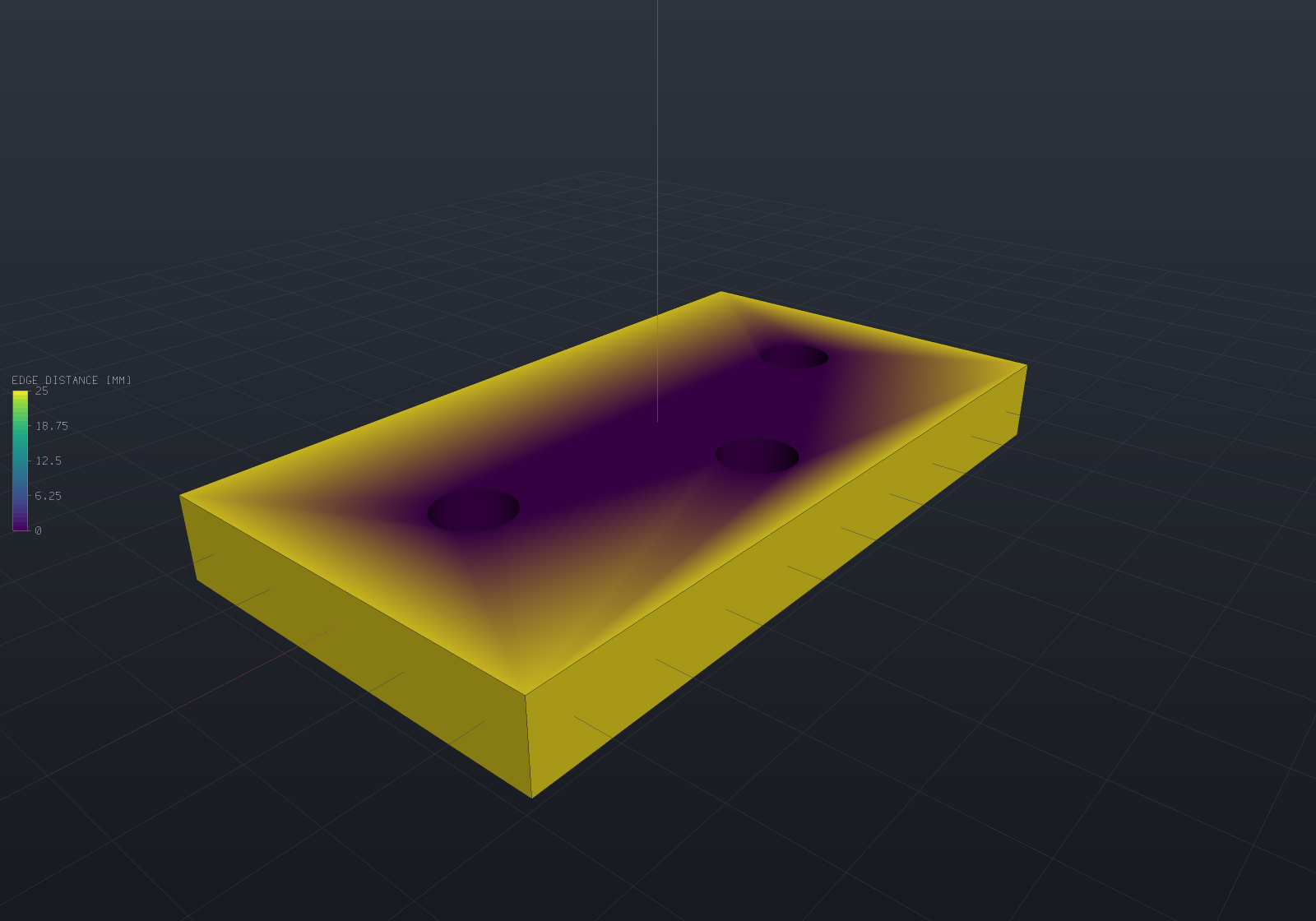

Run it in your browser

Three things are in that picture and all three come from the same handful of lines: the plate is painted through a perceptual colour map, the legend on the left states what the colours mean and over what range, and the range is the one the model asked for. Several visible parts showing genuinely different displays each get their own bar, stacked top-to-bottom in draw order (as many as fit vertically) — one bar over two scales would be a legend that lies — while parts sharing one display share one bar. Leave Range out and the field’s own min and max are used instead — which is the right default for a first look and the wrong one for a figure, since the bore walls sit at distance zero give or take a rounding error and the legend would say so.

Part.Results is a list, so a part can carry several and FieldDisplay names the one to show. Re-adding a result under an existing name replaces it, so re-running a solve updates the display instead of accumulating stale twins.

var part = new Part("plate", Shape.Box(40, 20, 4));
var mesh = part.GetMesh();

part.AddResult(MeshField.Sample(mesh, "von Mises", "MPa", p => 120 - 2 * Math.Abs(p.X)));
part.AddResult(MeshField.SampleVector(mesh, "displacement", "mm",
    p => new Vector3d(0, 0, -0.001 * p.X * p.X)));

if (part.Results.Count != 2) throw new Exception("both results should attach");

// A second result under the same name replaces the first (a re-solve, not a twin).
part.AddResult(MeshField.Sample(mesh, "von Mises", "MPa", _ => 0));
if (part.Results.Count != 2) throw new Exception("re-solving must not accumulate twins");
if (part.Result("von Mises")!.Range.Max != 0) throw new Exception("the live result should win");

Scalars, vectors and derived fields

A vector field (a displacement, a heat flux) reads as its magnitude wherever one number is wanted — colouring, the legend, the range — so FieldDisplay { Field = "displacement" } plots the deflection magnitude with no extra call. Magnitude() and Component(i) produce the derived field as an object of its own, for export or for its own legend.

var mesh = Shape.Box(10, 10, 10).ToMesh();
var u = MeshField.SampleVector(mesh, "displacement", "mm", p => new Vector3d(0, 0, p.Z * 0.1));

// ScalarAt is the magnitude for a vector field; the range follows it.
if (Math.Abs(u.Range.Max - 0.5) > 1e-9) throw new Exception($"range was {u.Range}");

var magnitude = u.Magnitude();          // named "|displacement|", same units
var uz = u.Component(2);                // named "displacement.Z"
if (magnitude.IsVector || uz.IsVector) throw new Exception("both derivations are scalar");

// The magnitude is unsigned by construction; a COMPONENT keeps its sign, which is
// exactly when the diverging map earns its keep.
if (magnitude.Range.Min < 0) throw new Exception("a magnitude cannot be negative");
if (Math.Abs(uz.Range.Min + 0.5) > 1e-9) throw new Exception($"uz should reach -0.5, was {uz.Range}");

The deformed shape

A displacement result can move the model, with the undeformed shape ghosted behind it, because the comparison is the point.

// A cantilever plate under an analytic deflection, exaggerated 40x. The colour is the
// deflection magnitude; the faint body behind it is the undeformed plate.
var part = new Part("cantilever", Shape.Box(120, 24, 6), Palette.Steel);
var mesh = part.GetMesh();

// A tip-loaded cantilever's shape: w(x) proportional to x^2 (3L - x), fixed at x = 0.
const double L = 120, tip = 0.35;
double Deflection(double x) => -tip * (x * x * (3 * L - x)) / (2 * L * L * L);

part.AddResult(MeshField.SampleVector(mesh, "displacement", "mm",
    p => new Vector3d(0, 0, Deflection(p.X + 60))));
part.FieldDisplay = new FieldDisplay
{
    Field = "displacement",     // a vector result colours by its magnitude
    Deform = "displacement",
    DeformScale = 40,           // real deflections are invisible; the legend states the factor
};

var scene = new Scene();
scene.Add(part);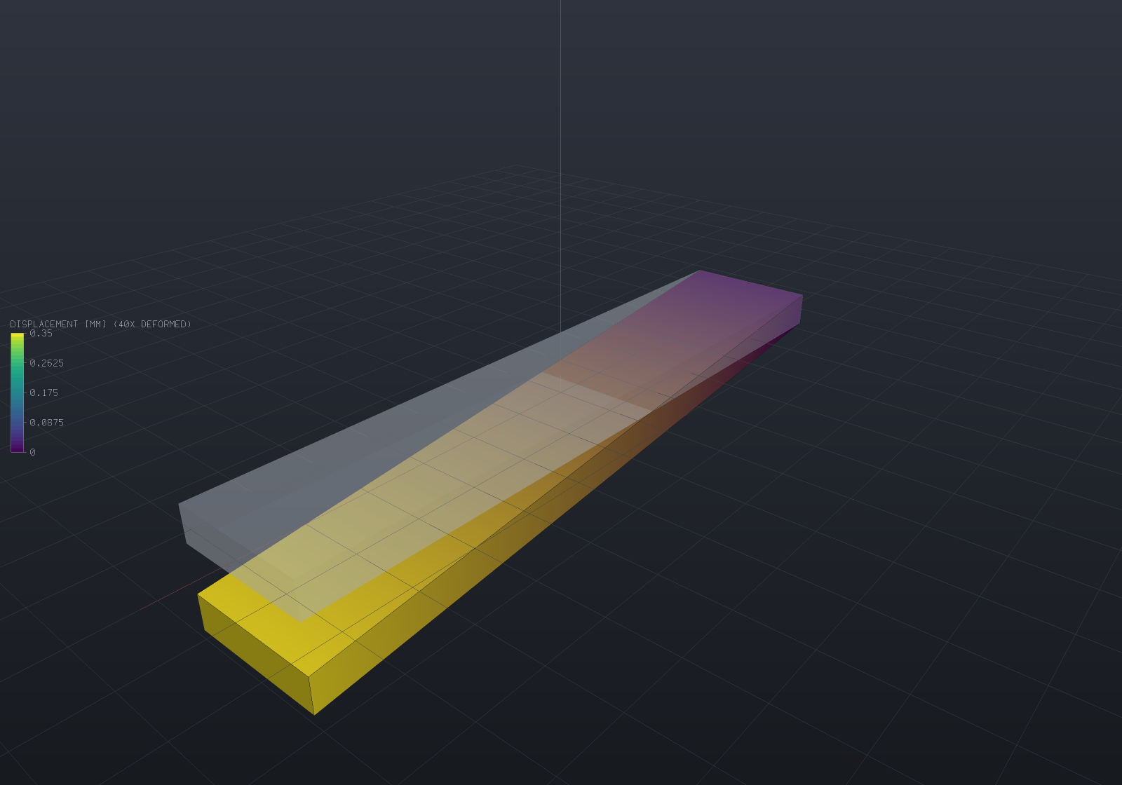

Run it in your browser

The legend’s title carries 40X DEFORMED, deliberately: a deformed plot whose exaggeration is not stated is a picture of a shape that does not exist. Set ShowUndeformed = false to drop the ghost, or DeformScale = 0 to leave the geometry alone entirely.

A deformed part draws its feature-edge overlay, displaced with the shape: each edge sample carries its own displacement (interpolated from the field at the sample’s nearest mesh facet — exact for any affine displacement, and within the facets’ own interpolation otherwise), riding a line-program attribute under the same uDeformScale the fills follow, so the outline is right at every exaggeration and animating it is still one float per frame. The wireframe view follows the displacement the same way — its endpoints are mesh vertices, so they take their own displacement vectors exactly. Picking follows what is drawn at the part’s own scale, so a click selects the part where it is on screen.

The displacement is sent once, as a vertex attribute, and the shader applies position + uDeformScale * displacement. A mesh with no displacement buffer reads zero, so a part with no results is untouched however the uniform is set — the same constant-when-absent rule the colour attribute follows. Two consequences worth knowing: the exaggeration is one float, so animating it is free (see the load ramp); and the shading is exact rather than carried over, because a facet normal is exactly quadratic in the scale, so three coefficients reproduce it at every exaggeration.

Every view style reads the field

A field-coloured part keeps its result colours in Wireframe and Points too: the wireframe’s segments take each endpoint’s own vertex colour (from the same mapping the fills use, so the two readings cannot disagree) and the point sprites read the mesh’s colour buffer directly. A part with no result keeps its part colour, exactly as before — and a cell-associated field keeps the part colour in wireframe, honestly: a mesh edge borders two faces, so an endpoint has no one cell colour to take.

// The edge-distance plate again, drawn as a wireframe: the mesh edges carry the
// field's colours, so the structure and the values read together.
var top = SketchPlane.At((0, 0, 5), Vector3d.UnitX, Vector3d.UnitY);
var plate = Shape.Box(90, 50, 10)
    .Drill(StandardHoles.Clearance(8), [new(-28, 0), new(0, 14), new(28, 0)], depth: 12, top);

var part = new Part("plate", plate) { DisplayMode = DisplayMode.Wireframe };
var mesh = part.GetMesh();

var bores = Sdf.Union(
    Sdf.Cylinder(4.5, 40).Translate((-28, 0, 0)),
    Sdf.Cylinder(4.5, 40).Translate((0, 14, 0)),
    Sdf.Cylinder(4.5, 40).Translate((28, 0, 0)));

part.AddResult(MeshField.Sample(mesh, "edge distance", "mm", p => bores.Evaluate(p)));
part.FieldDisplay = new FieldDisplay
{
    Field = "edge distance",
    Range = new FieldRange(0, 25),
};

var scene = new Scene();
scene.Add(part);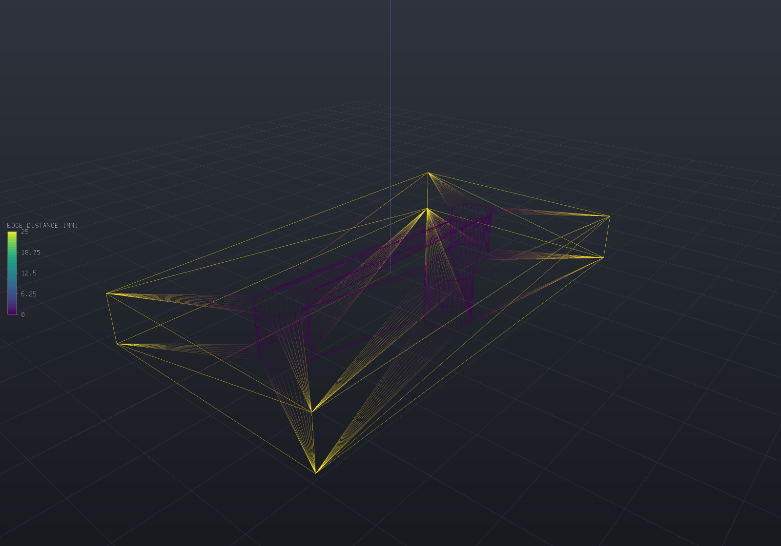

Run it in your browser

Transient playback

A transient run’s stored steps play back as a field-sequence track — the fifth animation slot, and the one whose sample is a result selection rather than matrices, a camera or a scalar. Steps are (result name, real seconds) pairs; t maps linearly over the run’s real span with hold-last-step semantics, because the stored states are the answers at their own instants — holding is honest where tweening colours between two solutions would invent a state the solver never produced. A part participates when it carries a display and all the run’s steps as results; the clip shows one range throughout (the display’s explicit range, else the union of the steps’ own), since a legend that rescales per frame lies. Applying a step re-uploads one colour buffer and nothing else — measured at 0.042/0.68 ms per frame on 12k/195k-vertex meshes — and a still of the animation at a step is byte-identical to a static render of the same configuration. The batched APNG/frame export applies the same rule per frame through the shared upload cache, and the browser viewer applies it through a colours-only buffer update — so an exported clip, the desktop window and the web viewer all play a transient run’s steps from one rule.

The axis itself is document data: Part.AddResultSequence publishes a run’s states as ordinary results under derived names (“T @ 0.5s”) and records a ResultSequence — the order and the instants — which persists with the document (write-only-when-stated, so a document using none is byte-identical) and from which FieldSequenceTrack.For builds the playback by one rule. A reloaded document then knows not just its states but WHEN they were; the track and the saved axis cannot disagree. A re-published sequence under the same name replaces the old one and removes any steps it no longer uses, so a re-solve with different instants cannot leave stale twins behind.

var part = new Part("plate", Shape.Box(20, 10, 2));
var mesh = part.GetMesh();

// Publish the run WITH its time axis: each step becomes a result named "T @ ...s",
// and the ResultSequence records the order and instants a saved document used to lose.
part.AddResultSequence("T", [
    (MeshField.Sample(mesh, "state", "K", p => 300 + p.X), 0.0),
    (MeshField.Sample(mesh, "state", "K", p => 300 + 4 * p.X), 5.0),
]);
part.FieldDisplay = new FieldDisplay { Field = "T @ 0s" };

var track = FieldSequenceTrack.For(part, "T");   // the saved axis IS the playback
if (track.FieldAt(0) != "T @ 0s" || track.FieldAt(1) != "T @ 5s")
    throw new Exception("t maps over the run's real time");
if (track.FieldAt(0.49) != "T @ 0s")
    throw new Exception("hold-last: 2.45 s still shows the 0 s step");

// The run's one range: the union of the steps' own.
var range = track.RunRange(part);
if (range.Min != 260 || range.Max != 340)
    throw new Exception($"the clip's range is the union, was {range.Min}..{range.Max}");

Colour maps and ranges

Two maps, and the choice matters:

FieldColorMap	For
Viridis (default)	A magnitude — stress, temperature, deflection — where only “more” and “less” mean anything. Monotone in lightness, so it survives greyscale printing and colour-vision deficiency.
Diverging	A signed quantity where the crossing is the interesting value. Blue–grey–red, with the neutral midpoint at the middle of the range.

A diverging map only means what it looks like over a range centred on zero, and EngrCAD will not silently re-centre one for you — quietly widening a range would change what the numbers on the legend say. Ask for it:

var mesh = Shape.Box(60, 20, 4).ToMesh();
var bending = MeshField.Sample(mesh, "bending stress", "MPa", p => 12 * p.Z);

var display = new FieldDisplay
{
    Field = "bending stress",
    ColorMap = FieldColorMap.Diverging,
    Range = bending.Range.SymmetricAboutZero(),   // so grey means zero
};

var range = display.Range!.Value;
if (Math.Abs(range.Min + range.Max) > 1e-12) throw new Exception("the range should straddle zero");
if (Math.Abs(range.Normalize(0) - 0.5) > 1e-12) throw new Exception("zero should land mid-map");

An explicit Range is also how several parts — or several load cases — are made comparable: without one, each field spans its own min and max and every picture gets its own private scale.

Two range behaviours are worth knowing. A constant field normalizes to 0.5 rather than to an end, because a field with no variation has no position to report and an extreme colour would read as a hot spot. And NaN is skipped when ranging, so one undefined value does not collapse a legend — and it paints a distinct neutral grey (ColorMaps.NoValueColor): NaN is “no value” (an infinite fatigue life, a part with no data in a merged export), not “small”, so it must not take the bottom of the ramp and read as the smallest finite value. When the displayed field carries a no-value node the legend adds a matching NO VALUE swatch below the bar; a finite field’s legend is unchanged. A LogScale display’s non-positive values land in the same grey for the same reason — a log scale has no position for them.

Log-scale fields

A field whose values are base-10 logarithms declares it in its units string — log10(cycles), the convention the fatigue life field established — and the legend reads that declaration: tick labels print the anti-logged values, ticks sit on the integer decades where the range spans at least two of them (with the end ticks always printing the true range), and the title states the base units with a LOG SCALE tag. The units string is the one opt-in, made by the field’s producer and carried by the field itself, so it round-trips wherever the field does; the colour mapping stays linear over the log values, which is exactly what a log colour axis is.

var life = MeshField.Scalar("life", "log10(cycles)", [2.0, 6.5, 10.0]);
if (!FieldLegend.TryLogUnits(life.Units, out var baseUnits) || baseUnits != "cycles")
    throw new Exception("the units string declares the log transform");

var display = new ResolvedFieldDisplay(
    life, new FieldRange(2, 10), FieldColorMap.Viridis, null, 1, true);
var ticks = FieldLegend.TickMarks(display);
if (ticks[0].Label != "100" || ticks[^1].Label != "1E+10")
    throw new Exception("ticks must print anti-logged values");
if (FieldLegend.Title(display) != "LIFE [CYCLES, LOG SCALE]")
    throw new Exception("the title must state the base units and the scale");

A field carrying real values that span decades (raw cycle counts, contact pressure) takes the other spelling: FieldDisplay.LogScale. The colour position becomes (log₁₀v − log₁₀min)/(log₁₀max − log₁₀min), so a value one decade up the range moves one decade up the ramp; a non-positive value has no log position and paints the no-value grey (NaN’s own convention); the legend prints the same decade ticks the units spelling prints for the same data — the two share one tick builder, so they cannot drift — and the title tags the field’s own units LOG SCALE. A log display needs a strictly positive range and is refused by name when it resolves otherwise; the flag rides in the document file write-only-when-set, so a file that never uses it is byte-identical. A display wants one spelling or the other, never both: the units string says the values are already logged, the flag says the colours should log them.

var life = MeshField.Scalar("life", "cycles", [10.0, 1e3, 1e5]);
var display = new ResolvedFieldDisplay(
    life, new FieldRange(10, 1e5), FieldColorMap.Viridis, null, 1, true, LogScale: true);

// 10^3 is the LOG midpoint of [10, 10^5] — linearly it would sit at t = 0.0099.
var colors = FieldRendering.SourceColors(life, display.Range, display.ColorMap, logScale: true);
if (colors[1] != ColorMaps.Sample(FieldColorMap.Viridis, 0.5))
    throw new Exception("the decade midpoint must take the map's middle colour");
if (FieldLegend.Title(display) != "LIFE [CYCLES, LOG SCALE]")
    throw new Exception("the title must tag the scale");

if (new FieldRange(4, 4).Normalize(4) != 0.5) throw new Exception("a constant field sits mid-map");
if (!FieldRange.Of([1, double.NaN, 5]).Equals(new FieldRange(1, 5)))
    throw new Exception("NaN must not poison a range");

// The colours the legend and the fills both use come from one call.
var cold = ColorMaps.Sample(FieldColorMap.Viridis, new FieldRange(0, 100), 0);
var hot = ColorMaps.Sample(FieldColorMap.Viridis, new FieldRange(0, 100), 100);
if (cold.B <= cold.R || hot.R <= hot.B) throw new Exception("viridis runs blue to yellow");

Exporting to ParaView (.vtu)

--export scene.vtu writes a VTK XML unstructured grid: the flattened instances’ geometry merged into one grid, plus every part’s results as point-data arrays.

var part = new Part("plate", Shape.Box(40, 20, 4));
var mesh = part.GetMesh();
part.AddResult(MeshField.Sample(mesh, "von Mises", "MPa", p => 40 + p.Z * 4));
part.AddResult(MeshField.SampleVector(mesh, "displacement", "mm",
    p => new Vector3d(0, 0, -0.002 * p.X * p.X)));

string path = Path.Combine(Scratch, "plate.vtu");
VtuWriter.WriteFile(mesh, part.Results, path);

var root = System.Xml.Linq.XDocument.Load(path).Root!;
if ((string?)root.Attribute("type") != "UnstructuredGrid") throw new Exception("wrong grid type");

var arrays = root.Descendants("PointData").Single().Elements("DataArray")
    .ToDictionary(e => (string)e.Attribute("Name")!, e => (string?)e.Attribute("NumberOfComponents"));
if (arrays["von Mises"] != "1") throw new Exception("stress should be a scalar array");
if (arrays["displacement"] != "3") throw new Exception("displacement should be a vector array");

The writer’s seam is deliberately (points, cells, cell types, point data) rather than a mesh type: a surface result writes triangles, quads and polygons today, and a volumetric mesher writes VtkCellType.Tetra through the same call with nothing in the writer changing.

When a scene merges several parts, the arrays are the union of their result names and a part that lacks one contributes NaN — VTK’s own “no value”, which ParaView paints in the map’s NaN colour. Dropping the array would lose the result that does exist, and zeros would show a fake safe region.

Where results fit in the document

Results live on the Part, not in a viewport. That is what makes them survive tab and scene plumbing, appear identically in the desktop window, a headless render and the browser client, and be visible to a script with no viewer reference at all.

Attaching a result is free and never meshes anything, so it does not interfere with Scene.PreMesh running parts in parallel. The one contract to keep is that a field’s values index the part’s display-mesh vertices, in vertex order — part.GetMesh().VertexCount of them. A field of the wrong length is reported by name when something tries to draw it, never silently ignored:

var part = new Part("plate", Shape.Box(10, 10, 10));
part.AddResult(MeshField.Scalar("stress", "MPa", [1, 2, 3]));   // far too short
part.FieldDisplay = new FieldDisplay { Field = "stress" };

// Resolution itself succeeds -- it does not mesh, deliberately, so a properties panel or
// an MCP tool can call it with no GL. The length check belongs to whatever draws it.
if (!part.TryResolveFieldDisplay(out var display, out _)) throw new Exception("should resolve");
if (display.Field.Count == part.GetMesh().VertexCount) throw new Exception("this field is short");

// A display naming a result that is not there fails loudly, and says what IS there.
part.FieldDisplay = new FieldDisplay { Field = "temperature" };
if (part.TryResolveFieldDisplay(out _, out string? error)) throw new Exception("should fail");
if (error is null || !error.Contains("stress")) throw new Exception("the error should list the results");

In the viewer the Fields toolbar toggle switches the whole thing off (every part back to its own colour and undeformed shape) and the properties panel shows the selected part’s results, the one being displayed, its range and any deformation scale — with a Result dropdown switching which result the part shows (the load-step/frequency selector in its honest discrete form: results are named states, so the control is a choice, not a range). Switching keeps the rest of the display — deformation, range, map — and it is one undoable edit through the same seam saving and MCP share. Headlessly, EngrCad.RenderToImage(scene, path, fields: false) does the same — which is how a geometry figure is taken of a model that also carries results.

Cell-associated fields

A field is vertex-associated by default, and interpolates across faces; a cell-associated field (MeshField.CellScalar, or the constructor’s FieldAssociation.Cell) carries one value per face — an element quality, a material id, a per-element stress — and renders flat on each. The association is part of the field’s identity: every derived operation (Magnitude, Component, Renamed, Scaled) preserves it, VtuWriter routes each field to PointData or CellData by it (counts validated against the right total), and the flat render mesh’s source-face map places a cell value on every duplicate of its face’s corners, so the flat look needs no shader change. A smooth render mesh shares vertices between faces, so it honestly carries no face map and a cell display on one refuses with the reason. A structural .vtu now carries the per-element von Mises as cell data beside the recovered nodal field — the value the assembly actually integrated, before any nodal recovery.