Modal analysis (natural frequencies)
EngrCAD.Fea finds a part’s natural frequencies and mode shapes on the same tetrahedral
meshes the mesher produces, with the same materials and the same supports
the structural solver already takes. It solves the generalized
eigenproblem
K·phi = lambda·M·phi, omega = sqrt(lambda), f = omega / 2·piby shift-and-invert Lanczos over one sparse Cholesky factorization, and publishes each mode shape as a field a viewer can colour by and deform.
var part = new Part("blade", Shape.Box(80, 20, 6));
// Meshing the PART's display mesh means the mode shapes land back on it exactly:// every display vertex is an analysis boundary node, matched by value.var surface = part.GetMesh();var tets = TetMesher.Mesh(surface, new TetMeshOptions{    RefineQuality = true,    MaxElementSize = 10,     // deliberately coarse - this page is a picture, not a study});
var model = new StructuralModel(AnalysisMesh.Of(tets), Materials.Steel);model.Fix(Facets.OnPlane(new Vector3d(-40, 0, 0), Vector3d.UnitX));
var results = ModalSolver.Solve(model, new ModalSolveOptions { ModeCount = 3 });
foreach (var field in results.SampleOnto(surface))    part.AddResult(field);part.FieldDisplay = new FieldDisplay{    Field = ModalResults.FieldNames.Shape(1),    Deform = ModalResults.FieldNames.Shape(1),    DeformScale = 8,};
var scene = new Scene();scene.Add(part);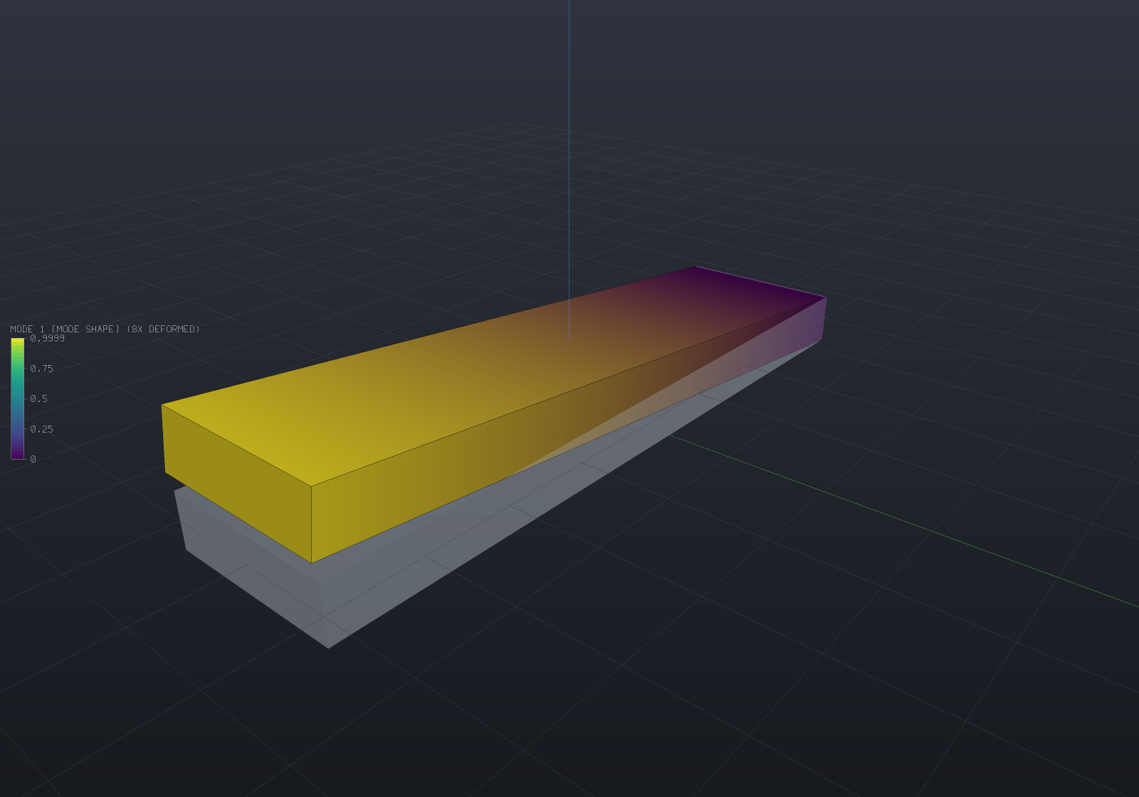
The shape is the first bending mode, drawn at a deliberate exaggeration with the undeformed
blade ghosted behind it. results.ToText() prints the frequencies, the effective masses and
what the solve cost.
Units, and why they come out in hertz
The mm / N / MPa / tonne / s system ModelUnits states once
(Materials & mass) is consistent in
seconds: one tonne is one N·s²/mm, so lambda = K/M has units
of 1/s² and omega and f come out in rad/s and Hz with no conversion. Use SI (m / N / kg)
and the same holds. Mix the two — a density in kg/m³ against a modulus in MPa — and the
frequencies are wrong by a factor of a thousand with nothing to catch it, which is why
ModalSolver refuses a zero density by name and quotes 7.85e-9 in the message.
Rigid-body modes are an answer, not an error
The static solver refuses an unrestrained body: a linear static solve of one has no unique answer, and it says which motions survive its supports rather than reporting a rank. A modal analysis of the same body is perfectly well posed, and its six zero-frequency modes are part of the answer — so the same machinery finds and describes them, and the modal solver keeps them:
var results = ModalSolver.Solve(model, new ModalSolveOptions { ModeCount = 3 });
foreach (var rigid in results.RigidBodyModes)    Console.WriteLine($"{rigid.Description}: {rigid.Frequency:E2} Hz");// translation along (1, 0, 0): 0.00E+000 Hz// rotation about the axis through (50, 6, 4) along (1, 0, 0): 9.82E-004 Hz// ...
Console.WriteLine(results.Mode(1).Frequency);   // the SEVENTH mode of the body
They are deliberately not part of Modes, and VibrationMode.Number starts at 1 on the
lowest mode that stores strain energy. Counting them among the structural modes is how a
report comes to claim a bracket’s first natural frequency is 3e-4 Hz.
Underneath, they are also deflated out of the Krylov space, so the eigensolver never
spends iterations rediscovering them; and because K is singular when they exist, the
factorization takes a small negative shift (ModalSolveReport.Shift, reported). A fully
restrained model needs no shift at all and the report says exactly zero — that
factorization is literally the static solver’s.
RigidBodyMode.Eigenvalue is the measured Rayleigh quotient of the exact rigid field.
In exact arithmetic it is zero; what it actually reads is how much round-off the assembled
stiffness carries, which makes it a conditioning measurement of that particular model rather
than a constant. Measured on the free-free beam below: the six values run from 3.8e-5 to
1.6e-3 against a first elastic eigenvalue of 6.8e8, i.e. 2.4e-12 of it at worst, and the
corresponding frequencies are all below 3e-3 Hz against 4 162 Hz.
Mode shapes have no amplitude and no sign
phi and −2.7·phi solve K phi = lambda M phi equally well, so a mode shape is a
direction in displacement space, not a displacement. Two conventions make the answer
reproducible without pretending otherwise:
VibrationMode.Shapeis mass-normalised (phi' M phi = 1). That is the scale every modal identity is stated in and the oneEffectiveMassneeds. Its magnitude is one over the square root of a mass, so it is not a displacement — plotting it directly would make a heavy part’s mode look small and would change if the density did.- The published field is rescaled to a peak nodal magnitude of exactly 1 model length
unit, and labelled
"mode shape"rather than"mm". SoDeformScale = 8means “the most-displaced node moves 8 mm”, which is a number a person can picture. - The sign is pinned by making the largest-magnitude component positive. Re-solving the same model twice gives the same vector, which is what an animation or a committed image needs — but the negated vector is an equally valid mode, and that is a convention rather than physics.
Field names are "Mode 1", "Mode 2", … through ModalResults.FieldNames.Shape(n). The
frequency is deliberately not in the name: a field name is a document-level handle that a
FieldDisplay stores and a saved document round-trips, and a name carrying a computed number
would stop resolving the moment a wall thickness changed.
The mass matrix
The mass matrix is the thermal solver’s capacity matrix under another
name — both are integral(constant · N_i · N_j dV) — so it is one implementation with rho
in place of rho·c, replicated onto the 3x3 identity block per node pair because an
isotropic inertia couples no two axes.
It needs a quadrature rule two degrees above the stiffness’s, and getting that wrong is
silent. A stiffness integrates grad N · grad N, degree 2(p−1); a mass integrates N·N,
degree 2p. Use the stiffness’s rule and an n-point rule gives a matrix of rank n — rank 1
of 4 for a linear element, rank 4 of 10 for a quadratic one, singular either way — while
sum_ij N_i N_j = (sum_i N_i)² = 1 exactly, so the total is still exactly rho·V. The
obvious sanity check passes it.
The negative control that has teeth is the rotational inertia. A rigid rotation is linear
in position, so both element orders represent it exactly and u' M u must equal the
tetrahedron’s own omega' I omega. Against MeshMassProperties’ closed-form polyhedral
moments — independent arithmetic in another project — the production rule agrees to
2.2e-16 … 9.4e-15 relative, while the stiffness’s one-point rule reports −2.4e-27
against a true 1.4e-10: no rotational inertia at all, because every entry being equal
collapses u' M u to the square of the mean nodal value and the mean of a rotation about the
centroid is zero.
Lumping
MassLumping | Available | What it buys |
|---|---|---|
Consistent | both orders (default) | the Galerkin matrix; converges at the element’s own order, from above |
Hrz | both orders | the consistent diagonal, rescaled to preserve the mass; converges from below |
RowSum | linear only | the textbook diagonal; identical to Hrz for a 4-node tet |
Row-sum lumping is refused by name for 10-node elements, because there it is not an
approximation but a wrong answer: a quadratic tetrahedron’s row sums are −V/20 at every
corner node — a negative mass, a node that accelerates towards a force pushing it away. It
is the same integral that makes a quadratic element’s consistent gravity load negative at the
corners, and no sign convention rescues it. HRZ takes the consistent matrix’s own diagonal,
rho·integral(N_i² dV), which is strictly positive for every shape function of every order,
and rescales it so the element’s mass is preserved.
The reason to offer a lumped option at all is not accuracy — it is that the two bracket the truth. Measured on a 16-element axial bar whose exact first frequency is 25 860.97 Hz:
| measured | error | |
|---|---|---|
| Consistent | 25 895.53 Hz | +0.134% |
| HRZ / row sum | 25 812.76 Hz | −0.186% |
Solving: this is where a direct factorization genuinely pays
FeaSolveMethod.Direct records, honestly, that the usual second argument for a direct solver
— factor once, solve many right-hand sides — does not apply to the static solver, which
factors and discards, so a second load case pays for a second factorization.
Here it applies. Shift-and-invert Lanczos factorizes K − sigma·M once and then spends
one back-substitution per Lanczos step. ModalSolveReport.Iterations says how many that
was, and it is the number that makes the argument concrete rather than rhetorical: on the
cases in this project’s test suite, 18 to 23 solves off a single factorization for three to
eight modes. No iterative linear solver is offered for the modal path for the same reason —
it would have to converge afresh for every one of those steps.
The operator is A^-1 M in the M inner product, whose eigenvalues are 1/(lambda − sigma),
so the frequencies nearest the shift become the largest of the operator — and extreme
eigenvalues are what Lanczos converges to first. Every new basis vector is re-orthogonalized
against every previous one (two passes), which is what stops round-off manufacturing spurious
duplicate eigenvalues.
That reorthogonalization creates its own problem, and the fix is worth knowing about because
it explains the restart count in the report. A single-vector Krylov space contains one
vector from each eigenspace, so a genuine multiplicity — a square shaft’s two identical
bending modes, every axisymmetric part — is invisible to it. Converged modes are therefore
locked: they join the deflation set, a fresh start vector is orthogonalized against them,
and the next run’s extreme eigenvalue is the second copy. For multiplicity three and above,
ModalSolveOptions.BlockSize advances a whole block of vectors per step so up to that many
copies are carried by construction (see the limitations below).
Verification
All of these are in tests/EngrCAD.Fea.Tests, on structured meshes (Kuhn’s subdivision)
so that a measured convergence order means something.
The axial bar, where there is no modelling gap
Every beam comparison below is against a beam theory, so its error is a discretization
error plus a modelling difference that no refinement removes. The bar fixture has
neither: with Poisson’s ratio exactly zero the axial and transverse directions decouple
completely, and with the transverse degrees of freedom removed the three-dimensional problem
is the one-dimensional one, whose free-free frequencies are n/(2L)·sqrt(E/rho) exactly.
100 mm steel bar, 40 linear elements, against n/(2L)·sqrt(E/rho):
| n | exact | measured | error |
|---|---|---|---|
| 1 | 25 861.0 Hz | 25 866.5 Hz | +0.021% |
| 2 | 51 721.9 Hz | 51 763.9 Hz | +0.081% |
| 3 | 77 582.9 Hz | 77 714.9 Hz | +0.170% |
Every one is above the exact value, and that is asserted as a strict inequality rather than a tolerance: a consistent-mass finite element model is a Rayleigh quotient over a subspace, so it can only be stiffer than the continuum.
Convergence order on the same bar, first mode, relative frequency error:
| linear | error | quadratic | error | |
|---|---|---|---|---|
| 8 elements | 5.479e-3 | 2 elements | 3.309e-3 | |
| 16 | 1.336e-3 | 4 | 1.885e-4 | |
| 32 | 3.317e-4 | 8 | 9.925e-6 | |
| 64 | 8.278e-5 | 16 | 5.691e-7 | |
| measured orders | 2.04, 2.01, 2.00 | 4.13, 4.25, 4.12 |
against theory 2 and 4 — an eigenvalue converges at O(h^2p) for a degree-p element.
The fixed-fixed version of the same bar has no rigid-body modes, so its shift is exactly zero and its errors are +0.025% / +0.095% / +0.194%.
Cantilever, 100 × 10 × 10 mm steel, quadratic elements
beta·L = 1.875104 / 4.694091 / 7.854757; the square section makes every bending mode a
degenerate pair, so the three bending modes are numbers 1, 3 and 7 (a torsional mode and
an axial mode fall between the second and third pairs).
| Euler-Bernoulli | measured | ||
|---|---|---|---|
| bending 1 (mode 1) | 835.5 Hz | 834.9 Hz | −0.07% |
| bending 2 (mode 3) | 5 236.1 Hz | 5 008.9 Hz | −4.34% |
| bending 3 (mode 7) | 14 661.2 Hz | 13 198.3 Hz | −9.98% |
The gap grows with the mode number, and that is beam theory rather than a solver error. Euler-Bernoulli has no shear deformation and no rotary inertia; a solid has both, and both soften it, increasingly so as the wavelength shortens while the section does not. Each measurement is asserted to be below Euler-Bernoulli for that reason, and the size is reported rather than tuned.
Refinement, first mode:
| mesh | elements | free DOF | measured | vs Euler-Bernoulli |
|---|---|---|---|---|
| 5×1×1 | 30 | 270 | 852.10 Hz | +1.985% |
| 10×2×2 | 240 | 1 500 | 838.30 Hz | +0.334% |
| 20×2×2 | 480 | 3 000 | 834.92 Hz | −0.071% |
| 30×3×3 | 1 620 | 8 820 | 833.78 Hz | −0.208% |
Monotone from above, which is again a theorem rather than an observation: a coarser mesh is a smaller subspace, so its Rayleigh quotient can only be larger. The sequence converges onto the 3D answer, which sits a little below the Euler-Bernoulli one — so the last row being further from the formula than the row above it is the study working, not failing.
The degenerate pairs split by 0.043% / 0.076% / 0.132%, and that split is a direct measurement of the discretization: the two bending directions are geometrically identical, but Kuhn’s subdivision picks its diagonals by index order and no reflection preserves that — the same asymmetry the static solver’s stress-concentration “mesh spread” measures.
Simply-supported beam, 100 × 12 × 8 mm
beta·L = n·pi. A rectangular section, so the two bending directions separate and each mode
can be identified with the beta·L it belongs to. This is the one case where the shear
correction has a closed form (the mode shape is a pure sine), so Timoshenko’s first-order
factor is quoted beside it:
| mode | beta·L | Euler-Bernoulli | Timoshenko | measured | vs EB | vs Timoshenko |
|---|---|---|---|---|---|---|
| 1 | 1·pi (weak) | 1 876.3 Hz | 1 856.2 Hz | 1 857.8 Hz | −0.98% | +0.09% |
| 2 | 1·pi (strong) | 2 814.4 Hz | 2 748.1 Hz | 2 751.5 Hz | −2.23% | +0.12% |
| 3 | 2·pi (weak) | 7 505.1 Hz | 7 199.3 Hz | 7 225.8 Hz | −3.72% | +0.37% |
| 4 | 2·pi (strong) | 11 257.6 Hz | 10 297.4 Hz | 10 361.7 Hz | −7.96% | +0.62% |
The 3D solve agrees with Timoshenko to under 0.7% at every mode while diverging from Euler-Bernoulli by up to 8% — which is the clearest statement available that the divergence belongs to the theory.
A finding this fixture cost, and it is worth stating because it is a modelling trap rather
than a solver one. The axial rigid translation has to be removed somehow, and the obvious
device — pinning u_x at a single node, exactly what a static 3-2-1 restraint does — is
wrong in dynamics. In statics a single-node restraint is a local disturbance Saint-Venant
confines to its own neighbourhood. In dynamics it creates a genuine mode in which the whole
body translates axially while a few elements around the pinned node deform, and its frequency
is set by the mesh rather than by the beam: measured on this fixture, a spurious mode at
5 540 Hz, sitting between the second and third bending modes and carrying 96% of the
axial effective mass. Holding u_x = 0 along the beam’s own centroidal line removes the
axial family instead, and adds no bending stiffness at all, because pure bending has
u_x = −z·w'(x) measured from the neutral axis and that is identically zero on it.
Free-free beam, 100 × 12 × 8 mm
No supports at all — the model the static solver refuses.
- Six rigid-body modes, three named as translations and three as located rotation axes. Measured eigenvalues −1.110e-3, 2.005e-4, −1.648e-3, 3.807e-5, −1.080e-4, 1.611e-4 against a first elastic eigenvalue of 6.84e8: at worst 2.41e-12 of it. The corresponding frequencies are all under 2.3e-3 Hz.
- The seventh mode is the first elastic one:
beta·L = 4.730041, Euler-Bernoulli 4 253.3 Hz, measured 4 162.1 Hz (−2.14%). The second is 6 379.9 Hz against 6 082.1 Hz (−4.67%).
Orthogonality
phi_i' M phi_j and phi_i' K phi_j assembled independently of the solver, element by
element, on a 6×2×2 cantilever with five modes:
worst abs(phi_i' M phi_j − delta_ij) | worst abs(phi_i' K phi_j − lambda_i·delta_ij) / lambda_i | |
|---|---|---|
| Linear | 7.105e-15 | 5.766e-13 |
| Quadratic | 7.550e-15 | 1.642e-11 |
Effective mass
Summed over all modes the effective masses recover iota' M iota exactly, which is what
makes “have I extracted enough modes?” a question with a numeric answer (the usual bar is
90%). A uniform cantilever’s first bending mode classically carries 0.6132 of the beam’s
mass; measured on the 100 × 12 × 8 quadratic cantilever, 61.09%.
On a square section that number splits in a way worth knowing about: modes 1 and 2 are degenerate, and the eigenvectors of a degenerate eigenspace are an arbitrary orthonormal basis of it, so each comes out as a mixture of the two bending directions and carries half the effective mass in each (measured: 2.399e-5 in Y and 2.399e-5 in Z, for both). A per-direction effective mass is therefore a property of an eigenspace, not of a mode, wherever the spectrum is degenerate.
Limitations
- These are UNDAMPED natural frequencies, which is what a modal analysis means. Damping, and the steady-state response it makes finite, are on the buckling and frequency response page.
- No transient dynamics. Direct time integration needs a different stepping loop, and is filed.
- Prestress is available but off by default. A spinning or preloaded part’s frequencies
shift, and
ModalSolveOptions.Prestressadds the geometric stiffness a static solve’s stress field produces — see stress stiffening. - Multiplicity three and above wants a BLOCK, and there is one.
ModalSolveOptions.BlockSize(default 1, the incumbent scalar path byte for byte) advances b vectors per Lanczos step, so a repeated eigenvalue of multiplicity up to b is recovered by construction — measured on synthetic exact triples and quadruples, where the scalar path returns{f1, f1, f2}for a truth of{f1, f1, f1}with every returned mode carrying a tiny residual (each IS an eigenpair, which is why nothing inside the iteration can notice a copy is missing). Set it to the largest multiplicity the model’s symmetry can produce; real meshes usually SPLIT their theoretical multiplicities, which is why 1 stays the default. - Sliver elements are the real constraint, and they belong to the mesher — refused by name here by the same shared guard both other solvers ask.