Structural analysis (linear static)

EngrCAD.Fea solves small-strain linear elasticity on the tetrahedral meshes the mesher produces: 4-node or 10-node elements, boundary conditions named through the same facet tags the mesher carries, a sparse symmetric solve on EngrCAD.Core.Solvers, and results published as fields that the viewer’s colour map and deformed-shape overlay pick up with no extra wiring.

The whole pipeline is five statements: mesh the surface, wrap it in a model, say what is held and what pushes, solve, publish.

var bracket = Shape.Box(60, 40, 10)
    .Subtract(Shape.Cylinder(6, 40).Translate(0, 0, -20));
var part = new Part("bracket", bracket);

// Meshing the PART's display mesh means the results land back on it exactly:
// every display vertex is an analysis boundary node, matched by value.
var surface = part.GetMesh();
var tets = TetMesher.Mesh(surface, new TetMeshOptions
{
    RefineQuality = true,
    MaxElementSize = 14,     // deliberately coarse - this page is a picture, not a study
});

var model = new StructuralModel(AnalysisMesh.Quadratic(tets), Materials.Aluminium6061);
model.Fix(Facets.OnPlane(new Vector3d(-30, 0, 0), Vector3d.UnitX));
model.Force(Facets.OnPlane(new Vector3d(30, 0, 0), Vector3d.UnitX), new Vector3d(0, 0, -1200));

var results = StructuralSolver.Solve(model);

foreach (var field in results.SampleOnto(surface))
    part.AddResult(field);
part.FieldDisplay = new FieldDisplay
{
    Field = StructuralResults.FieldNames.VonMises,
    Deform = StructuralResults.FieldNames.Displacement,
    DeformScale = 60,
};

var scene = new Scene();
scene.Add(part);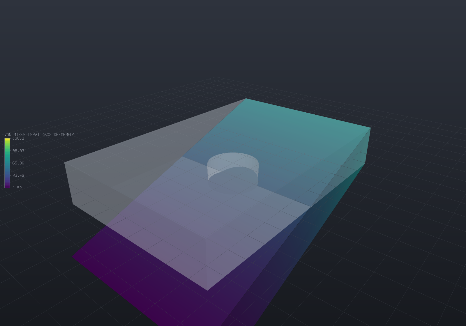

A bracket coloured by von Mises stress, drawn deformed — This example runs on the full kernel only — it uses TetMesher, which the browser build does not ship.

The bracket is fixed on its left face and pulled down by 1200 N on its right. The shape drawn is the deformed one at 60x exaggeration, ghosted over the original, and the colours are von Mises stress in MPa. The maximum is on the bore wall — measured, the peak node sits at radius 6.000 on a radius-6 hole — which is the classic stress concentration rather than the built-in edge an eye goes to first.

[!NOTE] That mesh is coarse on purpose, so this page builds in about four seconds. Its displacement is converged to under a percent but its peak stress is not — a concentration needs a much finer mesh at the feature. The verification numbers below are from the test suite, not from this picture.

Units

The mm / N / MPa / tonne / s system ModelUnits states once for the whole repository: lengths and displacements in mm, forces in N, stresses and moduli in MPa = N/mm² (steel E = 210 000), densities in tonne/mm³ (steel 7.85e-9), accelerations in mm/s² (Materials.GravityMillimetres = 9806.65). The quantity table and the reasoning behind the density choice are on the Materials & mass page — one statement, cross-referenced, rather than a copy per solver that could drift.

Saying what is held and what pushes

A boundary condition names a facet selector. Tags are the durable handle: pass B-Rep face ids through TetMeshOptions.FacetTags and a condition names a face rather than a coordinate, the way the rest of EngrCAD’s selection vocabulary works. The geometric selectors are for meshes that carry no tags — an imported STL, or a quick script.

Selector	Picks
`Facets.Tag(id)` / `Facets.Tags(...)`	Facets carrying those tags
`Facets.OnPlane(point, normal)`	Facets lying in a plane (centroid on it and normal parallel to it)
`Facets.FacingAlong(direction, angle)`	“The top surface”, “the loaded flank”
`Facets.InBox(aabb)`	Facets whose centroid is inside a box
`Facets.All`, `Facets.And`, `Facets.Or`	Everything, and the combinators

Condition	Meaning
`Fix(selector, dofs)`	A support. `Dof.All` clamps; `Dof.Z` alone is a roller
`FixNode(node, dofs)`	One node — how a statically determinate 3-2-1 restraint is built
`Prescribe(selector, displacement, dofs)`	An enforced deflection; the reaction is what a support at that displacement carries
`Pressure(selector, p)`	Uniform pressure. Positive pushes INTO the body
`Traction(selector, vector)`	Uniform force per unit area
`Force(selector, total)`	A total force spread over the selection — the resultant is exact
`Gravity(acceleration)`	Body load from the elements’ own material densities
`BodyForce(p => vector)`	A general body force per unit volume
`NodalForce(node, force)`	A point load (whose local stress does not converge — see below)

A selector that matches nothing is refused where it was written, naming the tags that do exist. A quietly ineffective support surfaces much later as a singular system, and the message there cannot point at the typo.

Several materials in one model

TetMesher tags each element with the index of the body it filled, and SetMaterial(region, material) assigns a material to a region id — a correspondence that is right only as long as two separately written lists stay in the same order. AnalysisBody makes it a fact rather than a convention: one list of (surface, material, name) drives both the mesh and the model, and it is also the seam with the document model, since a Part already knows both halves.

var steelBar = new Part("steel bar", Shape.Box(40, 6, 6).Translate(20, -6, 3))
    .Of(Materials.Steel);
var alloyBar = new Part("alloy bar", Shape.Box(40, 6, 6).Translate(20, 6, 3))
    .Of(Materials.Aluminium6061);

// The ONE list. Nothing below names a region id.
var bodies = new[] { steelBar, alloyBar }
    .Select(p => new AnalysisBody(p.GetMesh(), p.Material, p.Name))
    .ToList();

var tets = TetMesher.Mesh(bodies, new TetMeshOptions { RefineQuality = true, MaxElementSize = 3.0 });
var model = StructuralModel.For(tets, bodies);       // region i takes bodies[i].Material
model.Fix(Facets.OnPlane(new Vector3d(0, 0, 0), Vector3d.UnitX));
model.Force(Facets.OnPlane(new Vector3d(40, 0, 0), Vector3d.UnitX), new Vector3d(0, 0, -200));

var results = StructuralSolver.Solve(model);

double Tip(int side)
{
    double worst = 0;
    for (int n = 0; n < model.Mesh.NodeCount; n++)
    {
        var p = model.Mesh.Position(n);
        if (Math.Abs(p.X - 40) > 1e-9 || Math.Sign(p.Y) != side) continue;
        worst = Math.Min(worst, results.DisplacementAt(n).Z);
    }
    return -worst;
}

// A cantilever's deflection goes as 1/E, so the aluminium bar sinks about three times
// as far as its steel twin - measured 0.0756 mm against 0.2284 mm, a ratio of 3.02
// against the moduli's 3.05 (the small gap is that the mesher gave the two bars
// slightly different discretizations, not the materials).
double ratio = Tip(+1) / Tip(-1);
if (ratio < 2.9 || ratio > 3.2) throw new Exception($"expected ~3.05, got {ratio}");

ThermalModel.For reads the same list to the same answer, so a coupled run states what things are made of exactly once. Refused by name, before anything is assembled: a body with no material, a mesh region no body declares, and a declared body that contributed no elements.

[!IMPORTANT] v1 meshes DISJOINT bodies — two mating along a face are refused. Welding the shared vertices would mesh, and the result would look right and be wrong: an inter-body face is never recovered onto the input plane, so an element straddling the interface takes one material for its whole volume and the material boundary becomes a jagged surface of the mesher’s choosing rather than the plane that was drawn. Until conforming interfaces land, a bonded bi-material part is meshed as one surface with one material, and AnalysisBody serves genuinely separate bodies analysed together.

Directional materials — orthotropic and anisotropic

A laminate, a rolled plate and a printed part are all stiffer in one direction than another, and Material cannot say so: it is an isotropic description, and it lives in EngrCAD.Core because a bill of materials and a viewer need it too. ElasticLaw sits beside it rather than replacing it — the law supplies the elasticity (and, if it states one, the directional thermal expansion), while density, name and the thermal transport properties still come from the Material, so a modal solve of a composite part integrates the same density a BOM weighs it with.

The frame is the other half of the statement, and it is deliberately an input to the law rather than a property of the material: which way the fibres run in this part is not a property of the stuff.

// A unidirectional carbon/epoxy lamina - nominal figures, verify against a datasheet.
const double e1 = 135_000, e2 = 9_000, nu12 = 0.30, nu23 = 0.45, g12 = 4_800;

// Fibres at 30 degrees to the bar's axis, in the XY plane.
double angle = 30 * Math.PI / 180;
var fibreFrame = Frame3d.FromOrthonormal(
    Vector3d.Zero,
    new Vector3d(Math.Cos(angle), Math.Sin(angle), 0),
    new Vector3d(-Math.Sin(angle), Math.Cos(angle), 0));

var lamina = ElasticLaw.TransverselyIsotropic(fibreFrame, e1, e2, nu12, nu23, g12, "carbon UD");

var bar = new Part("bar", Shape.Box(40, 10, 4).Translate(20, 0, 0));   // x from 0 to 40
var tets = TetMesher.Mesh(bar.GetMesh(), new TetMeshOptions { RefineQuality = true, MaxElementSize = 3.0 });

// The Material still carries the density and the name; the law carries the stiffness.
var carrier = new Material("carbon UD", e1, 0.30, 1.6e-9);
var model = new StructuralModel(tets, carrier);
model.SetElasticity(0, lamina);

// Statically determinate: the whole end face held axially, then just enough more to
// remove the two transverse translations and the roll. A uniform uniaxial STRESS state
// satisfies all of it exactly, whatever the anisotropy.
const double sigma = 25.0;                       // MPa, a uniform end pull
model.Fix(Facets.OnPlane(Vector3d.Zero, Vector3d.UnitX), Dof.X);

int Corner(double y, double z)
{
    int best = -1;
    double bestScore = double.MaxValue;
    for (int n = 0; n < model.Mesh.NodeCount; n++)
    {
        var p = model.Mesh.Position(n);
        if (Math.Abs(p.X) > 1e-9) continue;
        double score = Math.Abs(p.Y - y) + Math.Abs(p.Z - z);
        if (score < bestScore) { bestScore = score; best = n; }
    }
    return best;
}

model.FixNode(Corner(-5, -2), Dof.Y | Dof.Z);
model.FixNode(Corner(+5, -2), Dof.Z);
model.Traction(Facets.OnPlane(new Vector3d(40, 0, 0), Vector3d.UnitX), new Vector3d(sigma, 0, 0));

var results = StructuralSolver.Solve(model);
var strain = results.ElementStrain(0);
double apparent = sigma / strain.Xx;

// The classical off-axis modulus: 1/Ex = c^4/E1 + s^4/E2 + (1/G12 - 2 nu12/E1) s^2 c^2.
double c2 = Math.Cos(angle) * Math.Cos(angle), s2 = Math.Sin(angle) * Math.Sin(angle);
double classical = 1.0 / (c2 * c2 / e1 + s2 * s2 / e2 + (1.0 / g12 - 2.0 * nu12 / e1) * s2 * c2);

// 20 267 MPa - a seventh of the fibre-direction stiffness, at 30 degrees off axis.
if (Math.Abs(apparent - classical) > 1e-6 * classical)
    throw new Exception($"expected {classical:F1} MPa, got {apparent:F1}");

// And the bar SHEARS under a pure pull, which is the behaviour no isotropic law has.
if (Math.Abs(strain.Xy) < 1e-3 * Math.Abs(strain.Xx))
    throw new Exception("an off-axis lamina must show shear-extension coupling");

Three factories, in increasing generality:

	states	for
`ElasticLaw.TransverselyIsotropic`	5 constants + frame	a unidirectional lamina, a drawn bar, a printed part’s layer stack
`ElasticLaw.Orthotropic`	9 constants + frame	a woven laminate, a rolled plate, wood
`ElasticLaw.Anisotropic`	the 6x6 matrix + frame	anything else, including a homogenised microstructure

The minor Poisson’s ratios are derived from the symmetry nu_ji / E_j = nu_ij / E_i rather than taken as inputs — supplying both is how a datasheet transcription comes to contradict itself, and the contradiction would make the matrix non-symmetric with nothing to catch it. What is checked, by name, is that the compliance matrix is positive definite: the classical restriction |nu_ij| < sqrt(E_i / E_j) plus a determinant condition coupling all three is that statement, and a Cholesky is the statement rather than a re-derivation of it. Without the check a plausible-looking transcription gives a material that releases energy when strained, and the symptom is a factorization failure deep in the solver rather than a message about the material.

Thermal expansion is directional too, and it is stated on the law:

var withExpansion = lamina.WithThermalExpansion(fibreFrame, -0.5e-6, 28e-6, 28e-6);

An expansion stated on the law always wins over the Material’s scalar coefficient, and a directional region that states none is refused by name rather than inheriting one — the scalar route builds its load from the material’s Lamé parameters, which are not that region’s stiffness at all, so the inherited number would have no well-defined meaning. Rotating a directional expansion off its own axes produces genuine shear terms (a heated off-axis lamina shears), which is why the free strain is carried as a six-component vector rather than three numbers.

[!NOTE] An isotropic model is untouched by all of this, deliberately and provably: the assembly branches on ElasticLaw.IsIsotropic, so a model that states no law assembles through exactly the arithmetic it did before — bit for bit, asserted — while the general B'DB path is separately asserted to agree with the index form to round-off on an isotropic law. Anisotropy costs nothing until it is asked for, and cannot silently change what a plain steel bracket reports.

Modal, buckling, harmonic and transient solves all read the same law, because they all assemble their stiffness through FeaAssembly.

Reading the answer

var plate = Shape.Box(50, 30, 8);
var part = new Part("plate", plate);
var surface = part.GetMesh();
var tets = TetMesher.Mesh(surface, new TetMeshOptions { RefineQuality = true, MaxElementSize = 12 });

var model = new StructuralModel(AnalysisMesh.Of(tets), Materials.Steel);
model.Fix(Facets.OnPlane(new Vector3d(-25, 0, 0), Vector3d.UnitX));
model.Force(Facets.OnPlane(new Vector3d(25, 0, 0), Vector3d.UnitX), new Vector3d(0, 0, -800));
model.Gravity(Materials.GravityMillimetres);

var results = StructuralSolver.Solve(model);
Console.WriteLine(results.Report.ToText());
Console.WriteLine($"peak von Mises {results.MaxVonMises:F2} MPa at node {results.MaxVonMisesNode}");
Console.WriteLine($"largest displacement {results.MaxDisplacement:F4} mm");

// Global force equilibrium must hold to round-off for ANY correct model - it is the
// cheapest end-to-end check there is, and nothing about it is visible in a stress plot.
if (results.Report.EquilibriumResidual > 1e-9)
    throw new Exception($"equilibrium residual {results.Report.EquilibriumResidual:E3}");

// ParaView, for anything the viewer does not show.
results.WriteVtu(Path.Combine(Path.GetTempPath(), "plate.vtu"));

FeaSolveReport is a value, not a log line: sizes, factor fill, timings per phase, the solve residual, strain energy, the applied and reaction resultants, and the equilibrium check. StructuralSolveOptions.EstimateCondition adds a power-iteration estimate of the stiffness matrix’s condition number — the number that tells a badly shaped mesh from a badly posed model.

Beyond the report, StructuralResults gives nodal Displacement, averaged NodalStress and NodalVonMises, per-material NodalStressIn/NodalVonMisesIn, PrincipalStress, per-element ElementStress/ElementStrain, and Reactions. Element values are kept public on purpose: the nodal values are a volume-weighted average of the elements meeting at a node, which is what a colour map wants and what converges — and it also smooths a genuine discontinuity at a material interface or a re-entrant corner. The jump between neighbouring elements is the standard error indicator, and averaging is the standard way to hide a mesh that is too coarse.

Is the mesh good enough? Stress recovery and the error estimate

A solve returns a number whatever the mesh. StructuralResults.ErrorEstimate is the answer to whether that number is worth anything — the energy-norm gap between the element stress field and its superconvergent recovery, per element and overall.

The premise is where the stress is sampled. A displacement-based element’s stress is one order lower than its displacement and jumps across faces, and inside the element it is most accurate at the Gauss points and least accurate at the nodes — which is where a colour map reads it. StressRecovery.Superconvergent fits a polynomial to the good points over each patch of elements and evaluates it at the nodes.

var part = new Part("bracket", Shape.Box(50, 30, 8));
var tets = TetMesher.Mesh(part.GetMesh(), new TetMeshOptions { RefineQuality = true, MaxElementSize = 6 });

var model = new StructuralModel(tets, Materials.Steel);
model.Fix(Facets.OnPlane(new Vector3d(-25, 0, 0), Vector3d.UnitX));
model.Force(Facets.OnPlane(new Vector3d(25, 0, 0), Vector3d.UnitX), new Vector3d(0, 0, -400));

var results = StructuralSolver.Solve(model);

double direct = results.MaxVonMises;
results.Recovery = StressRecovery.Superconvergent;
double recovered = results.MaxVonMises;

var estimate = results.ErrorEstimate;
Console.WriteLine(estimate);                       // "estimated error 12.4% (...)"
Console.WriteLine($"peak {direct:F1} -> {recovered:F1} MPa");

// The per-element map is what the adaptive refinement loop below consumes.
int worst = estimate.WorstElement;
Console.WriteLine($"worst element {worst}, error {estimate.ElementError[worst]:E3}");

if (estimate.ElementError.Count != model.Mesh.ElementCount) throw new Exception("one value per element");
if (double.IsNaN(estimate.RelativeError)) throw new Exception("this mesh has interior nodes, so it must estimate");
if (!(estimate.RelativeError > 0)) throw new Exception("a coarse mesh should report some error");

Direct remains the default: every verification figure in this project was measured through it, and a recovered field is smooth by construction, so at a genuine discontinuity — a re-entrant corner, where the true stress is singular — it smooths harder than averaging does. Recovery is a better answer for the common case, not a better answer.

A material interface used to be the other example on that list and no longer is. A patch is never fitted across one: patches are assembled from the elements of a single region, so a node on the interface carries one recovered value per material rather than one wrong value for both. That matters more than the smoothing plain averaging does because of reach — averaging blends the shared node and nothing else, while a patch is written to every node of every element it contains, so one cross-interface fit puts a ramp into nodes a whole element layer inside each material. Measured on a bi-material cube whose exact stress is piecewise constant: 34 single-material nodes wrong, the worst by 92.9%, against exact to 4.5e-15 with the rule.

// One value per node - so at an interface node this is the average of the materials.
var blended = results.NodalStress[node];

// The honest per-material value. Equal to the above, bit for bit, at any node touching one
// region; refused by name at a node touching no element of that region.
foreach (int region in model.Mesh.RegionsAt(node))
    Console.WriteLine($"region {region}: {results.NodalVonMisesIn(region, node):F1} MPa");

// How many nodes the node-indexed field blends. Zero for a single-material part and for
// disjoint bodies, which share no node.
Console.WriteLine($"{model.Mesh.InterfaceNodeCount} interface nodes");

[!NOTE] No mesh the public API can build has an interface node yet. TetMesher meshes disjoint bodies and refuses two that mate along a face, so no node is ever shared between two materials — the per-region recovery is a precondition for conforming interfaces rather than a fix to something reachable today, and InterfaceNodeCount is currently zero everywhere.

[!IMPORTANT] The estimate reports NaN, not zero, when it cannot estimate. A mesh with no interior corner node has no patch to fit, so the “recovered” field is the finite-element field and the arithmetic gives the distance from something to itself — measured on a 24-element box, 9.9e-15 against a true error of 0.313. That would call the mesh perfect on exactly the mesh too coarse to assess. ErrorEstimate.FallbackNodes counts the partial case for the same reason: a recovery that quietly did not happen must not look like one that did.

AdaptiveSolve.Run closes the loop the estimate opens: solve, estimate, make the elements smaller where the error is large and larger where it is small, re-mesh, repeat. The rule is the classical one, h_new = h_old * (target/e_local)^(1/p) for an equidistributed error, with p the element degree because that is the energy-norm rate.

You hand it a closed surface and a callback that builds the model on whatever mesh a round produces. The callback shape is what the loop needs — a StructuralModel is bound to one AnalysisMesh and every round has a new one — and it is sound because boundary conditions are named by Facets selectors rather than by facet indices.

var surface = Shape.Box(40, 20, 8).ToMesh();

var result = AdaptiveSolve.Run(
    surface,
    mesh =>
    {
        var model = new StructuralModel(mesh, Materials.Steel);
        model.Fix(Facets.OnPlane(new Vector3d(-20, 0, 0), Vector3d.UnitX));
        model.Force(Facets.OnPlane(new Vector3d(20, 0, 0), Vector3d.UnitX), new Vector3d(0, 0, -400));
        return model;
    },
    new AdaptiveOptions
    {
        TargetRelativeError = 0.15,
        MaxRounds = 2,
        MaxElements = 25_000,
        Mesh = new TetMeshOptions { MaxElementSize = 8 },
    });

Console.WriteLine(result.ToText());

// The answer is an ordinary solve on the final mesh.
double tip = result.Results.MaxDisplacement;
Console.WriteLine($"tip {tip:F4} mm at {result.RelativeError * 100:F1}% estimated error");

if (result.Rounds.Count < 1) throw new Exception("a run always reports its rounds");
if (result.Rounds[^1].RelativeError > result.Rounds[0].RelativeError)
    throw new Exception("refining must not make the estimate worse");
if (!(tip > 0)) throw new Exception("the final round is a real solve");

What it buys, measured

The comparison that means anything is uniform refinement of the same model, by the same mesher and solver, to the same estimated error. Measured on a 24 x 5 x 5 cantilever (AdaptiveRefinementTests, win-x64), starting from 1 764 elements at 39.48%:

	elements	estimated error	peak/mean element error
adaptive, round 1	9 406	22.49%	4.14
uniform, size 1.4	11 410	23.50%	6.68
uniform, size 1.2	18 049	20.46%	7.04
uniform, interpolated to 22.49%	13 204	22.49%	—

The uniform arm’s own rate over that ladder measures error ~ N^-0.271. Linear tetrahedra converge at N^-0.333 on a smooth problem, so a rate below it is the fixture reporting that the clamp singularity really is what limits it — which is both the calibration the interpolation needs and the check that the comparison is running on the right problem. It is asserted, not just printed, with the bound being the theory constant rather than a tuned number.

[!NOTE] That rate is fitted over the whole ladder, and a two-point rate would not do. The ladder is not a refinement sequence — the mesher’s red-refinement overshoot sets the element counts, so the rungs jump unevenly and the pairwise rates swing 0.2235 to 0.3776, two of them above 1/3. Interpolating the headline ratio still uses the local bracketing pair, which is what interpolation wants and is measurably insensitive here (1.40x to 1.48x across the plausible range); asserting a fixture property does not.

So 1.40x fewer elements at the same estimated error, and the reason is the last column: the error is spread 1.6x more evenly over the adapted mesh, so no small group of elements is holding the global figure up. The refinement goes where the singularity is — over the five millimetres nearest the clamp the mean element size fell to 0.439 of its starting value, while over the five nearest the tip it fell to 0.989, which is to say the tip was left alone.

[!NOTE] peak/mean does not fall monotonically with every round on a singular fixture, and that is honest rather than a defect. Halving an element far from the clamp roughly halves its error; halving one at the clamp barely moves it. So a round that refines both lowers the global figure and widens the spread. The claim that survives is the matched-cost one above.

Two knobs that are not tuning

SizeGradation bounds how fast the requested size may change with distance. It is not a smoothing nicety: the raw field is piecewise constant over the old elements, so a refined region meets an unrefined one at a cliff, and a mesher asked to put a 0.4 mm element against a 3 mm one across one face answers with slivers. Measured with the limit off on a raw MeshPrimitives box — already the mesher’s worst-case surface — the next round’s conjugate-gradient solve did not converge at all (13 185 free DOF, 250 s, the estimate coming back at 100%); with it, the same round solves in the ordinary way. On a remeshed surface the same defect is milder and still one-signed: 9 060 elements at 23.36% unlimited against 9 406 at 22.49% limited — a bigger mesh for a worse answer. The direction generalises; the magnitude belongs to the surface.

ReductionPerRound aims a round at max(target, measured x factor) rather than at the final target every time. Without it a far target makes every element’s ratio fall below MinRefineFactor, the whole mesh clamps to one factor, and the run pays a uniform refinement’s bill for an adaptive scheme’s complexity. It sets how big a round is rather than how much a round is worth: 0.5 / 0.7 / 0.85 gave 13 284 / 9 406 / 7 373 elements at 20.30% / 22.49% / 24.76%, which against that fixture’s own uniform rate (error ~ N^-0.30) all sit on one curve.

Stopping is a decision

A model with a genuine singularity never reaches an arbitrary target, so the loop caps its rounds and reports the figure it stalled at rather than refining forever — the same shape as boundary recovery’s non-convergence detection. AdaptiveResult.Outcome says which cap it hit: Converged, RoundsExhausted, Stalled (a round that did not improve on the one before) or ElementBudgetExceeded (the next mesh’s predicted size, from the sizing field itself, over MaxElements — checked before paying for the mesh that would prove it).

Refused by name: a target outside (0, 1), a non-positive round budget, a first mesh already over the element budget, a callback that returns a model over a different mesh, a solve that did not converge, and a mesh so coarse that no recovery patch exists — refining against a NaN estimate would be refining against nothing.

Elements

	Linear (4-node)	Quadratic (10-node)
Built by	`AnalysisMesh.Of(tets)`	`AnalysisMesh.Quadratic(tets)`
Strain within an element	constant	linear
Integration	1 point (exact)	4 points, degree 2 (exact for straight-sided elements)
Nodes	the mesh’s vertices	vertices + one per edge, about 7-8x as many
Displacement convergence	O(h²)	O(h³)
Energy convergence	O(h)	O(h²)

Quadratic elements are worth their cost for anything involving bending or a stress concentration, and the tables below say by how much. QuadraticTetMesh is a pure function of the linear mesh — mid-edge nodes at exact midpoints, so elements stay straight-sided, which is what makes the 4-point rule exact.

Solving

The default is sparse Cholesky with an AMD fill-reducing ordering, and that ordering is not a micro-optimisation. On a 6 552-DOF 10-node cantilever it cut the factor from 19.4 million entries to 1.7 million and the factor time from 64.8 s to 0.34 s — 11.3x less fill and 191x faster — because fill is what decides whether a quadratic solve is practical at all.

FeaSolveMethod.ConjugateGradient is the alternative, and the honest measurement is that it usually wins — by a lot, on anything big. Interleaved in one sitting (Release):

	free DOF	direct	CG	winner
linear	2 160	247 ms	122 ms	CG 2.0x
linear	14 688	10 754 ms	705 ms	CG 15.3x
linear	46 800	108 459 ms	2 232 ms	CG 48.6x
quadratic	6 552	308 ms	354 ms	direct 1.1x
quadratic	14 688	2 688 ms	1 094 ms	CG 2.5x

That is the opposite of the crossover measured on a Laplacian, which is the point: such a comparison measures the operator’s conditioning, not the two algorithms.

The direct solver keeps the default because it is exact, not because it is fast. The verification numbers below — a patch test reproduced to round-off, strain at 1e-13 — are statements that cannot be made about an iterative solve stopped at a relative residual, and a default of CG would make every one of them a claim about an opt-in path. Pass ConjugateGradient for a large single solve; past ~15 000 unknowns it is not close. No automatic size-based switch is offered, deliberately: a threshold taken from one cantilever would be the same mistake the table above documents.

You do not have to remember that, though — the report tells you. When a direct factorization both takes real time and dominates its own solve, FeaSolveReport.Advisory says what this run spent where and what the benchmark measured at a comparable size, and ToText() prints it. It fires on what happened, not on size: a system that factors quickly stays silent however large it is.

Several load cases at once

The other classic argument for a direct solver — factor once, substitute many right-hand sides — is what SolveAll exists for. Build every case over one AnalysisMesh object, vary the loads (and prescribed values, if you use them), and the assembly and factorization happen once:

var cases = loads.Select(f =>
{
    var m = new StructuralModel(mesh, Materials.Steel);
    m.Fix(Facets.Tag(1));
    m.Force(Facets.Tag(2), f);
    return m;
}).ToList();

var results = StructuralSolver.SolveAll(cases);

Measured against the same cases solved one at a time (Release, alternating in one sitting): 3.5–3.8x for four cases and 6.9x for eight, because an extra right-hand side costs 0.7–27 ms where the factorization costs 34–4 706 ms. It also moves the direct-vs-iterative comparison, since CG reuses nothing and would pay for N whole runs.

What the cases must share — the mesh object, the restraint mask, the materials — is checked and refused by name. That matters more than it sounds: pushing one case’s loads through another’s factorization returns a displacement field that converges, passes its own residual check, and is the answer to a different model.

A SolveAll pair is also exactly what fatigue post-processing consumes: the two extremes of a duty cycle, decomposed into per-node alternating and mean stress.

Watching, and stopping

That advisory helps the second run and not the first, so every solve entry point also takes Core’s optional trailing ProgressCancel:

using var source = new CancellationTokenSource();   // wire this to a Cancel button
var watch = new ProgressCancel(source.Token, fraction => Console.WriteLine($"{fraction:P0}"));

var results = StructuralSolver.Solve(model, null, watch);

Cancellation reaches SparseCholesky.Factorize’s per-column elimination loop, which is the only thing that makes the parameter honest — the factorization is 99% of a slow solve, so a cancellation that could not reach it would advertise something it cannot do. It reaches the conjugate-gradient path too, and the transient thermal stepper.

The fraction is the factorization’s own, and that is a measurement rather than a shortcut: on any model slow enough to want a progress bar the factorization is the solve. Inside it the fraction counts work, not columns — a factor that fills has done only about an eighth of its arithmetic at the halfway column. Assembly and the reaction pass poll for cancellation but report no fraction, and an iterative solve reports none at all, because an iteration count is not progress.

Supports are eliminated, not penalised: constrained degrees of freedom are removed from the system rather than given a large diagonal, so the reduced matrix is genuinely positive definite and its conditioning is the model’s own.

Refusals

An unrestrained body is refused before the factorization, per connected body, with the surviving motion described rather than counted:

The model is not restrained: 3 rigid-body modes survive the supports
(rotation about the axis through (10, 7.5, 5) along (1, 0, 0); ...).
1 node is restrained in all. A linear static solve of an unrestrained body has no
unique answer; add supports, or restrain the six rigid-body degrees of freedom
statically (a 3-2-1 scheme) if the loads are self-equilibrated.

The check is per connected body, because a fully fixed part beside a floating one is singular in a way no whole-model rigid mode describes. Letting the factorization discover it instead gives “nonpositive pivot at column 4713”, which tells nobody anything.

Also refused by name: a selector matching no facets; a model with every degree of freedom restrained; an element whose Jacobian is non-positive in double precision (which a sliver can be while the exact predicate still calls it valid — see the limitations below); and a Poisson’s ratio at or past 0.5, where the material is incompressible and a displacement-based element cannot represent it.

Verification

A solver is worth exactly what its verification is worth, so here is all of it. Every number is from tests/EngrCAD.Fea.Tests, on structured meshes so that a measured convergence order means something.

Patch tests — a constant-strain state must be reproduced exactly, to round-off, by both element types. This is the standard correctness gate and it catches essentially every assembly, indexing and Jacobian error outright.

Test	Linear	Quadratic
Displacement patch: relative displacement error	2.4e-15	1.8e-14
Displacement patch: relative strain error	9.1e-14	1.5e-13
Traction patch: stress error against 25 MPa	3.9e-12	1.1e-11
Traction patch: relative displacement error	4.0e-14	2.5e-13

Convergence order (manufactured solution, cubic displacement field, Dirichlet everywhere — no singularity for the rate to be limited by):

	L2 order measured	theory	energy order measured	theory
Linear	2.00	2	1.00	1
Quadratic	3.03	3	2.02	2

Cantilever tip deflection, 100 x 10 x 10 mm, 1000 N tip load, steel:

	h	elements	tip (mm)	error
linear	5.00	192	0.55157	-71.0%
linear	2.50	1 536	1.15880	-39.2%
linear	1.25	12 288	1.63297	-14.3%
quadratic	10.00	24	1.81094	-4.9%
quadratic	5.00	192	1.87899	-1.4%
quadratic	2.50	1 536	1.89778	-0.4%

Euler-Bernoulli PL³/3EI gives 1.90476 mm; Timoshenko, adding the shear term PL/(kGA) with k = 5/6, gives 1.91962 mm. The extrapolated finite-element limit is 1.90494 mm — +0.01% from Euler-Bernoulli and -0.76% from Timoshenko.

That near-perfect agreement with the simpler beam model is a coincidence of two effects cancelling, and saying so is the point: a 3D solve includes shear deformation, which softens it towards Timoshenko, while the built-in end here is a genuine three-dimensional clamp — every displacement zero over that whole face — which suppresses the Poisson contraction and warping beam theory allows and stiffens it back. Note also that linear tetrahedra are very stiff in bending: 14% low with twelve thousand elements, against 0.4% for quadratic elements with an eighth as many.

Stress concentration, a 120 x 40 x 2 mm plate with a Ø10 central hole (d/W = 0.25) in plane strain:

	elements	K_tn measured	vs Howland
linear	768	1.8352	-24.6%
linear	3 072	2.1941	-9.8%
linear	12 288	2.3566	-3.1%
quadratic	768	2.3206	-4.6%
quadratic	3 072	2.4216	-0.4%

Kirsch’s classical answer for an infinite plate is K_t = 3. The finite-width correction matters and has to be stated: Howland’s exact strip solution in Peterson’s polynomial fit (Chart 4.1), against the net section stress, is K_tn = 2 + 0.284L - 0.600L² + 1.32L³ with L = 1 - d/W, which at d/W = 0.25 gives 2.4324 — equivalently 3.2432 against the gross section, nearly 8% above the textbook 3. The far-field stress is recovered to 0.03% on the finest quadratic mesh and 0.37% on the coarsest linear one, which is the check that makes every K_t above mean anything.

Stress recovery — the claim is a rate, so it is measured as an L2 norm of the nodal stress field against the exact one, integrated inside the elements over a refinement sequence on the same manufactured solution:

	direct	recovered	direct rate	recovered rate
linear, 12 288 el	2.302e-2	1.599e-3	1.418	2.300
quadratic, 1 536 el	2.669e-3	2.348e-4	2.000	2.761

against theory 1/2 and 2/3 — 14.4× and 11.4× more accurate, at a clearly higher rate. The quadratic rate settling near 2.76 rather than 3.00 is reported as measured: full p+1 recovery on tetrahedra is weaker than on hexahedra. The effectivity index (estimated over true error, energy norm) runs 0.9544 → 0.9848 → 0.9955 for linear elements and 1.0187 → 1.0150 → 1.0128 for quadratic — monotone toward 1 from below and above — and a linear stress field is recovered exactly (1.1e-12 of 3.2e2) with the estimated error 0.00%.

Directional materials, all exact rather than converging — a uniform stress state in a prismatic bar is a constant strain, hence a linear displacement field, which is in the linear-tetrahedron space:

	measured	reference
off-axis lamina at 0°	135 000.00 MPa	E1 exactly
at 30°	20 267.42 MPa	classical `1/Ex = c⁴/E1 + s⁴/E2 + (1/G12 - 2ν12/E1)s²c²`
at 45°	12 406.66 MPa	same, agreeing to 1e-12 relative
at 90°	9 000.00 MPa	E2 exactly

with the whole strain tensor reproduced to 4.4e-17 against a 2.0e-3 scale and the uniform stress state to 1.4e-12 of 25 MPa. The expected strain is built by 3x3 tensor rotation — rotate the stress into the material frame, apply the compliance there, rotate the strain back — which shares nothing with the production path’s Voigt stress transformation but the physics; the classical modulus formula is then a third reading of the same number. The shear-extension coupling is asserted separately (−7.9e-4 at 30°, exactly zero on axis), because it is the one behaviour no isotropic law can produce and the one a transposed rotation would lose. Directional expansion: a free bar strains by exactly alpha_i·dT (1.1e-17 of 1.7e-3) with residual stress at 1.2e-13 of the 15.12 MPa a restrained bar would carry, and a fully restrained bar carries σ = (−12.72, −27.95, −27.95) MPa — three genuinely different numbers — to 3.6e-15.

Rigid-body and equilibrium properties, all satisfied to round-off:

Every element’s stiffness annihilates all six rigid-body modes (both orders).
A rigid motion prescribed on the boundary produces a rigid motion inside, with strain at 1e-14 of the field’s own scale and energy at 1e-15 of a comparable straining motion’s.
A self-equilibrated load gives identical strains (4.6e-13 relative) and identical strain energy under two different statically determinate 3-2-1 restraints, with both reactions at 1e-13 of the applied load.
The whole answer is frame-indifferent: strain energy and peak von Mises agree to 1e-12 when the model, its loads and its supports are rigidly placed somewhere else.
Gravity reacts the body’s exact weight; a uniform pressure over a closed surface has no resultant; a total force distributed over a face set sums back to itself exactly.
The two element orders agree on strain energy to twelve digits wherever both reproduce the field exactly.

Limitations

Sliver elements are the real constraint, and they belong to the mesher. The Delaunay mesher’s own README names sliver removal as its top quality gap, and a structural solve is where it bites: measured on a 100 x 10 x 10 beam at a 5.0 size target, 32% of the elements are slivers below 10°, two have a non-positive double-precision volume, and the factorization fails outright. The solver refuses those by name rather than absorbing them. Compact bodies mesh well; long thin ones do not yet.
Element-associated results have nowhere to go. MeshField is vertex-only in v1, so a per-element stress cannot be exported or displayed directly; ElementStress is available in code.
Stress at a quadratic element’s nodes is evaluated directly rather than extrapolated from the integration points; StressRecovery.Superconvergent is the opt-in that does the latter (above).
A material interface is a per-node answer a per-node field cannot hold. The recovery never fits across one and NodalStressIn gives each material’s own value, but the published MeshFields and .vtu still carry the blended node value, so a colour plot smooths the interface. Unreachable today — no mesh the public API builds has a shared node between two materials.
No contact, no plasticity, no large deformation. Every one of those is a different mathematical problem rather than a bigger version of this one. Modal analysis has landed and reuses this assembly unchanged — see natural frequencies and mode shapes.