Transient dynamics (direct time integration)

TransientSolver steps the equation of motion

M·a + C·v + K·u = f(t)

forward in time by the Newmark / HHT-alpha family, over the same tetrahedral meshes the mesher produces, the same materials, and the same supports and load selectors the structural solver takes. It answers “what does this structure do next” for an arbitrary load history — a suddenly applied force, an impact, a ramp, a shaker trace — where modal analysis answers “what does it like to do” and harmonic response answers “what does it do under a steady sine”.

The one number everybody wants: dynamic amplification

A load applied suddenly deflects a structure roughly twice as far as the same load applied slowly. That factor is exactly 2 for an undamped single oscillator, and a real part lands near it. Here is a steel plate cantilevered from one end with a tip load switched on at t = 0:

var part = new Part("plate", Shape.Box(80, 20, 5));

// Meshing the PART's display mesh means the results land back on it exactly:
// every display vertex is an analysis boundary node, matched by value.
var surface = part.GetMesh();
var tets = TetMesher.Mesh(surface, new TetMeshOptions
{
    RefineQuality = true,
    MaxElementSize = 10,     // deliberately coarse - this page is a picture, not a study
});

var mesh = AnalysisMesh.Of(tets);
var clamped = Facets.OnPlane(new Vector3d(-40, 0, 0), Vector3d.UnitX);
var tip = Facets.OnPlane(new Vector3d(40, 0, 0), Vector3d.UnitX);

StructuralModel Case() =>
    new StructuralModel(mesh, Materials.Steel)
        .Fix(clamped)
        .Force(tip, new Vector3d(0, 0, -400));

// The natural period sets the step: 40 steps per cycle of the mode being excited.
var modes = ModalSolver.Solve(
    new StructuralModel(mesh, Materials.Steel).Fix(clamped),
    new ModalSolveOptions { ModeCount = 1 });
double period = 1.0 / modes.Mode(1).Frequency;

// The prose below quotes this band; asserting it here is what keeps the two from drifting.
if (modes.Mode(1).Frequency is < 300 or > 3000)
    throw new Exception($"first mode {modes.Mode(1).Frequency:F0} Hz is outside the quoted band");

var results = TransientSolver.Solve(
    Case(), new TransientSolveOptions(period / 40, 120));

// The instant of largest deflection, and the same load solved statically.
var peak = results.States[0];
foreach (var state in results.States)
{
    if (state.MaxDisplacement > peak.MaxDisplacement)
        peak = state;
}
var statics = StructuralSolver.Solve(Case());

double amplification = peak.MaxDisplacement / statics.MaxDisplacement;
if (amplification < 1.7 || amplification > 2.1)
    throw new Exception($"dynamic amplification {amplification:F3} is not near 2");

foreach (var field in peak.Results.SampleOnto(surface))
    part.AddResult(field);
part.FieldDisplay = new FieldDisplay
{
    Field = StructuralResults.FieldNames.Displacement,
    Deform = StructuralResults.FieldNames.Displacement,
    // The camera frames the UNDEFORMED bounds, so an exaggeration large enough to
    // push the tip outside them would crop the picture.
    DeformScale = 12,
};

var scene = new Scene();
scene.Add(part);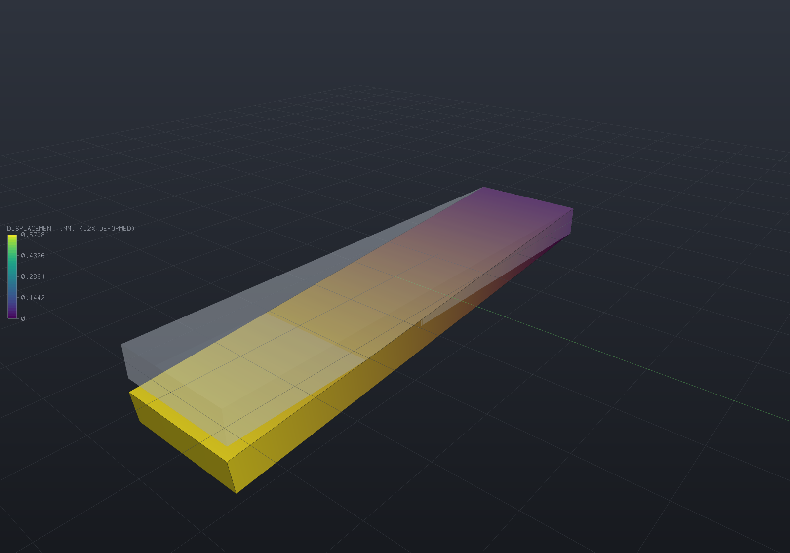

This example runs on the full kernel only — it uses StructuralModel, which the browser build does not ship.

The shape is the plate at the peak of its first swing, drawn at a deliberate exaggeration with the undeformed plate ghosted behind it. The peak deflection is close to twice the static one, and the plate then oscillates about the static position for ever — because nothing here is damped.

On the time scale, honestly. This plate’s first bending mode is a few hundred hertz, so the three cycles above span a few milliseconds. A transient of a stiff metal part is always like that — hundreds of hertz to tens of kilohertz — so if you animate one you are watching a slowdown of a thousand or more, and the caption should say so rather than implying the clip runs at true speed. Only structures like buildings and long spans are slow enough to watch honestly. (It is the same caveat DeformationTracks.Oscillate carries for a mode shape, and the one readers most often assume a solver has arranged away.)

Choosing a step

There is no stability limit to respect — every scheme this solver will construct is unconditionally stable (see what is refused) — so the step is chosen purely on accuracy, and the quantity that decides it is omega·dt for the highest mode you care about.

Newmark’s default member has an exactly known error: its algorithmic frequency is omega·(1 - (omega·dt)²/12), so a mode resolved at N steps per period runs slow by (2·pi/N)²/12 and the phase falls behind by 2·pi·(2·pi/N)²/12 radians per period. That is the whole error budget for a linear problem:

steps per period	period error	phase lag after 10 cycles
20	0.82%	0.52 rad (30°)
40	0.21%	0.13 rad (7.4°)
100	0.033%	0.021 rad (1.2°)
200	0.0082%	0.0052 rad (0.3°)

Twenty to forty steps per period of the highest mode that carries real energy is the usual engineering choice. Note what the table is not: it says nothing about modes the step cannot resolve, which is the next section.

Numerical damping, and why the default has none

A finite element mesh has as many modes as degrees of freedom, and the top ones are discretization artefacts — they have no physical content and no physical damping. Newmark’s default member is neutrally damped: it preserves the amplitude of every mode exactly, artefacts included, which is what makes its energy identity exact and also what leaves that numerical noise ringing through the whole run.

TimeIntegration.ForSpectralRadius(rho) selects the HHT member that multiplies the amplitude of an unresolvable mode by rho each step:

var neutral = TimeIntegration.ForSpectralRadius(1.0);
var damped = TimeIntegration.ForSpectralRadius(0.8);

// rho = 1 IS Newmark's average acceleration, by value.
if (neutral != TimeIntegration.AverageAcceleration)
    throw new Exception("a neutral spectral radius should be the default member");

// Both are second order - which is the whole point of HHT over a raised Newmark gamma.
if (!damped.IsSecondOrder || !damped.IsUnconditionallyStable)
    throw new Exception("HHT should keep second order and unconditional stability");

// The relation is alpha = (rho - 1)/(rho + 1).
if (Math.Abs(damped.Alpha - (0.8 - 1) / (0.8 + 1)) > 1e-15)
    throw new Exception("unexpected alpha");

The three families available, and what each costs:

scheme	order	high-frequency amplitude per step	use it when
AverageAcceleration (default)	2	1 — nothing decays	you want the exact energy identity, and the mesh’s top modes are not being excited
ForSpectralRadius(rho) / HilberHughesTaylor(alpha)	2	rho, chosen	an impact, a contact-like step change, or any load that rings the mesh
NumericallyDamped(gamma)	1	falls with gamma	you specifically want Newmark’s own amplification; otherwise HHT is strictly better

Two rules worth stating. gamma = 1/2 exactly is what makes a Newmark member second order, so NumericallyDamped trades an order for its damping and says so in its own name. And HHT’s dissipation is aimed at omega·dt large — a well-resolved mode is barely touched, which is the property that makes it safe to leave on.

Damping

RayleighDamping gives C = alpha·M + beta·K, fitted the way anyone actually picks it — two frequencies and two ratios:

var damping = RayleighDamping.FromRatios(
    frequency1: 500, ratio1: 0.02,
    frequency2: 5000, ratio2: 0.02);

// A U-shaped curve: the fitted points are met, and everything between them is damped LESS.
if (Math.Abs(damping.RatioAtFrequency(500) - 0.02) > 1e-12)
    throw new Exception("the fit should meet its first point");
if (damping.RatioAtFrequency(1581) >= 0.02)
    throw new Exception("the minimum sits between the fitted points");

// Outside the fitted range it damps MORE - often much more, which is the trap.
if (damping.RatioAtFrequency(50_000) < 0.05)
    throw new Exception("a stiffness-proportional term over-damps the high end");

For this proportional run option no damping matrix is assembled. Every appearance of C is either a product C·x = alpha·(M·x) + beta·(K·x) — two matrix-vector products the solver already performs — or a scalar multiple that folds into the effective stiffness as (…)·M + (…)·K. Forming C would cost a third sparse matrix with the stiffness’s sparsity and buy an operation more expensive than the two products it replaces.

Damping that is not proportional — a discrete dashpot, per-region coefficients that differ — is carried on the model rather than the run option, because it is geometry-attached data:

model.Dashpot(nodeIndex, new Vector3d(0, 0, 1), coefficient: 5.0);  // grounded viscous damper

When a model carries damping the transient assembles C once (the one matrix the project builds, shared with the direct harmonic solver) and folds it into the effective stiffness and every step’s right-hand side. It composes additively with the proportional run option, and a model that states no damping assembles nothing — so the common Rayleigh path is unchanged. Hysteretic (structural) damping is a different model still — frequency-domain by definition (i·eta·K, a complex modulus) with no causal time-domain form — and belongs to the direct harmonic solve rather than to time integration.

What none of these routes gives is the damped natural modes of a non-proportionally damped system: that is the quadratic eigenproblem (lambda²M + lambda·C + K)phi = 0, a 2n-dimensional non-symmetric state-space problem whose modes are complex. Nothing here attempts it — but the steady-state RESPONSE (DirectHarmonicSolver) and the transient RESPONSE (here) both need no such modes.

Initial conditions

A run starts from rest unless told otherwise. InitialDisplacement and InitialVelocity are per node of the analysis mesh (which for quadratic elements includes the mid-edge nodes), and the initial acceleration is solved for:

a(0) = M⁻¹·(f(0) - C·v(0) - K·u(0))

That is a solve against M, not against K, and it is the second factorization a run pays for. It matters: a body released from a displaced position, or one whose load is already on at t = 0, is accelerating at that instant, and starting from a(0) = 0 instead puts a spurious half-step into the answer whose symptom — a startup wobble that decays — looks exactly like physics.

The value of the load history at t = 0 is yours. A step written with g(0) = 1 starts the body accelerating immediately; written with g(0) = 0 it starts at rest and the first step applies the load. Both are legitimate readings of “suddenly applied”.

One factorization for the run

The step is constant, and that is a design decision rather than a simplification: the stepping matrix a0·M + (1+alpha)·a1·C + (1+alpha)·K depends on the step, the scheme and the model and on nothing else, so it is factored once before the loop and every step after that is a back-substitution. TransientSolveReport.Factorizations reports the count — one for the stepping matrix, plus one for the mass matrix when the initial acceleration has to be solved. A continuously varying step would refactor at every change, which is the entire cost of the method — so adaptive stepping, when you want it, uses a small fixed set of sizes and factors each once.

Base excitation (support motion)

A shaker table or a seismic input drives the model through its supports, not by a nodal force. TransientSolveOptions.BaseMotion states it as a ground ACCELERATION a_g(t) along a direction, and the answer is RELATIVE displacement — measured from the moving base, which is the right quantity for stress because a rigid ground motion carries none. In relative coordinates the equation is M·u'' + C·u' + K·u = -M·iota_d·a_g(t), so it is one more inertial load pattern over the supports left fixed — no per-step operator change, and it takes the acceleration a seismic record already is:

var tets = TetMesher.Mesh(Shape.Box(60, 12, 8).ToMesh(), new TetMeshOptions
{
    RefineQuality = true,
    MaxElementSize = 12,
});
var mesh = AnalysisMesh.Of(tets);
var model = new StructuralModel(mesh, Materials.Steel)
    .Fix(Facets.OnPlane(new Vector3d(-30, 0, 0), Vector3d.UnitX))
    .Force(Facets.OnPlane(new Vector3d(30, 0, 0), Vector3d.UnitX), new Vector3d(0, 0, -200));

// A shaker table: the whole base accelerates as a_g(t) along Z. It COMPOSES with the model's
// own load (the tip force), so this is gravity-held-while-shaken in one run.
var options = new TransientSolveOptions(2e-6, 200)
{
    Damping = RayleighDamping.StiffnessProportional(30000, 0.05),
    LoadFactor = t => 1.0,
    BaseMotion = new BaseMotion(Vector3d.UnitZ, t => 9810 * Math.Sin(2 * Math.PI * 20000 * t)),
};
var shaken = TransientSolver.Solve(model, options);
if (!shaken.IsRelativeToBase)
    throw new Exception("a base-motion run reports RELATIVE displacement");

// A ZERO base motion is the plain force-driven run, bit for bit - the feature is off by default.
var still = TransientSolver.Solve(
    model, options with { BaseMotion = new BaseMotion(Vector3d.UnitZ, _ => 0.0) });
var plain = TransientSolver.Solve(
    model, new TransientSolveOptions(2e-6, 200) { Damping = options.Damping, LoadFactor = t => 1.0 });
for (int i = 0; i < plain.States.Count; i++)
    for (int n = 0; n < mesh.NodeCount; n++)
        if (BitConverter.DoubleToInt64Bits(still.States[i].DisplacementAt(n).Z)
            != BitConverter.DoubleToInt64Bits(plain.States[i].DisplacementAt(n).Z))
            throw new Exception("a zero base motion must match a plain run bit for bit");

The relative form is kept over prescribing the absolute support motion because it is measured to be the same physics and cleaner (design.md §3g): the two agree to 6.1e-12 on an undamped problem, and the relative response matches the transmissibility amplification 1/sqrt((1-r²)² + (2·zeta·r)²) to 0.075% and the resonant 1/(2·zeta) to 0.062%. The whole base moves together (independent foundations are a larger construction, stated not detected).

Adaptive time stepping

The constant step is what lets one factorization serve the run, so the adaptive form must not give that away. SolveAdaptive draws its step from a small DYADIC set — TimeStep / 2^L for L in 0..Levels-1 — and factors each size at most ONCE, cached, so a multi-scale run (a sharp start then a long ring-down) spends the fine step only where a local-error estimate demands it while paying for at most Levels factorizations, not one per step change:

var tets = TetMesher.Mesh(Shape.Box(60, 12, 8).ToMesh(), new TetMeshOptions
{
    RefineQuality = true,
    MaxElementSize = 12,
});
var mesh = AnalysisMesh.Of(tets);
var model = new StructuralModel(mesh, Materials.Steel)
    .Fix(Facets.OnPlane(new Vector3d(-30, 0, 0), Vector3d.UnitX))
    .Force(Facets.OnPlane(new Vector3d(30, 0, 0), Vector3d.UnitX), new Vector3d(0, 0, -200));
var transient = new TransientSolveOptions(2e-6, 200)
{
    Damping = RayleighDamping.StiffnessProportional(30000, 0.1),
    LoadFactor = t => 1.0,
};

// Levels == 1 is the constant-step Solve reproduced bit for bit through the SAME step
// arithmetic, with the same factorization count - the seam that pins it as a strict extension.
var constant = TransientSolver.Solve(model, transient);
var oneSize = TransientSolver.SolveAdaptive(
    model, transient, new TransientAdaptiveOptions { Levels = 1, Tolerance = 1e9 });
if (oneSize.Report.Factorizations != constant.Report.Factorizations)
    throw new Exception("a single-size adaptive run factors the same matrices");
for (int i = 0; i < constant.States.Count; i++)
    for (int n = 0; n < mesh.NodeCount; n++)
        if (BitConverter.DoubleToInt64Bits(oneSize.States[i].DisplacementAt(n).Z)
            != BitConverter.DoubleToInt64Bits(constant.States[i].DisplacementAt(n).Z))
            throw new Exception("Levels == 1 must reproduce the constant run bit for bit");

// Three sizes {dt, dt/2, dt/4}: at most one factorization per size (plus the mass solve),
// NOT the ~thousand a continuously varying step would do.
var adaptive = TransientSolver.SolveAdaptive(
    model, transient, new TransientAdaptiveOptions { Levels = 3, Tolerance = 5e-6 });
if (adaptive.Report.Factorizations > 3 + 1)
    throw new Exception("adaptive factors at most one matrix per size, not one per step change");
_ = adaptive.Report.AdaptiveSteps;    // total steps taken
_ = adaptive.Report.StepsPerLevel;    // the split between the sharp start and the ring-down

Measured on the verification suite, a damped free decay whose amplitude falls ~1000x is matched to the uniform-fine reference to 0.008% while taking 816 steps against the fine grid’s 1920 (58% fewer) and factoring 4 matrices (three sizes plus the mass solve). The tolerance is absolute, so set it to the response’s own scale; the split is dramatic only when the ring-down genuinely goes quiet (an under-damped run oscillates the whole time at the natural frequency).

The energy balance is an identity, not a diagnostic

TransientSolveReport.EnergyBalanceResidual measures

|(E_final - E_initial) - WorkDone + Dissipated|

relative to the magnitudes involved. For the default scheme this is exact algebra, damped and loaded cases included. The trapezoidal update relations give u(n+1) - u(n) = (dt/2)(v(n) + v(n+1)) and v(n+1) - v(n) = (dt/2)(a(n) + a(n+1)), from which

E(n+1) - E(n) = (dt/4)·(v(n)+v(n+1))'·[M(a(n)+a(n+1)) + K(u(n)+u(n+1))]

and putting the equation of motion at both ends into the bracket turns it into exactly the work and dissipation terms. Nothing is approximated, so a drift there is a defect rather than a tolerance — measured on this project’s fixtures, 4.4e-13 relative over 3000 steps.

For a dissipative scheme the same number becomes the measurement instead of the check: it is the energy the algorithm removed, which is what a user of numerical damping wants reported. Integration.IsSecondOrder and Integration.SpectralRadiusAtInfinity say which case a run is in.

What a run gives back

TransientResults carries every stored state (StoreEvery thins them), and each TransientState is a full StructuralResults — so stress, von Mises, field publishing and .vtu export all work per instant — plus the velocity, the acceleration and the energies:

var tets = TetMesher.Mesh(Shape.Box(60, 12, 8).ToMesh(), new TetMeshOptions
{
    RefineQuality = true,
    MaxElementSize = 12,
});
var mesh = AnalysisMesh.Of(tets);
var model = new StructuralModel(mesh, Materials.Steel)
    .Fix(Facets.OnPlane(new Vector3d(-30, 0, 0), Vector3d.UnitX))
    .Force(Facets.OnPlane(new Vector3d(30, 0, 0), Vector3d.UnitX), new Vector3d(0, 0, -200));

var results = TransientSolver.Solve(
    model,
    new TransientSolveOptions(2e-6, 100)
    {
        Damping = RayleighDamping.MassProportional(2000, 0.03),
        StoreEvery = 5,
        LoadFactor = t => 1.0,       // a step, held
    });

var final = results.Final;
_ = final.Velocity;                  // per node
_ = final.Acceleration;              // per node
_ = final.KineticEnergy;             // ½ v'Mv
_ = final.StrainEnergy;              // ½ u'Ku
_ = final.Results.MaxVonMises;       // stress recovery, per instant
_ = results.DisplacementHistory(0);  // one node over the whole run
_ = results.At(1.0e-4);              // the nearest STORED instant, never interpolated

// The energy balance holds as an identity even with damping and a load present.
if (results.Report.EnergyBalanceResidual > 1e-10)
    throw new Exception($"energy balance {results.Report.EnergyBalanceResidual:E2}");

// Global equilibrium in d'Alembert's form: applied + reaction = inertia + damping.
if (results.Report.WorstEquilibriumResidual > 1e-9)
    throw new Exception($"equilibrium {results.Report.WorstEquilibriumResidual:E2}");

At(time) returns the nearest stored state rather than interpolating, deliberately: an interpolated displacement satisfies neither the equation of motion nor the scheme’s own update relations, so it would be a plausible field with no provenance.

Verification

Every figure below is measured by the test suite, and every prediction it is compared against is derived rather than quoted.

The single oscillator

A model whose reduced system is exactly 1 x 1 — every degree of freedom restrained but one — so there is no discretization error at all and every difference belongs to the time integrator. Its stiffness comes from a static solve and its frequency from a modal solve, so the references are never the transient’s own arithmetic.

case	closed form	measured
step load, dynamic amplification	exactly 2	2.0000
damped step, zeta = 5%	1.8544679	1.8544825
free vibration, 10 periods at 100 steps/period	2.067% phase error	2.014%
initial velocity (impulse)	2.067%	2.066%
damped step response, worst error	0.06051% of static	0.06058%
damped free vibration, worst error	0.1513% of u0	0.1513%
harmonic drive at r = 0.8, zeta = 5%	closed-form magnification	0.027%
the same, against HarmonicSolver	—	0.027%

The phase-error predictions are the algorithmic-frequency result stated above: after N periods the displacement error is amplitude · 2·pi·N·(omega·dt)²/12, and for a damped run that product peaks at t = 1/(zeta·omega) with value amplitude·(omega·dt)²/(12·zeta·e).

Energy

case	expected	measured
undamped free vibration, 50 periods (3000 steps)	conserved exactly	4.4e-13 relative drift
largest excursion at any step of that run	—	5.2e-13
damped + loaded, work 1.44 and dissipation 6.28	balance is an identity	1.4e-13
rho_inf = 1 at omega·dt from 0.1 to 1000	amplitude preserved	1.0 to 1e-11

Convergence in time

scheme	theory	measured
Newmark (1/4, 1/2)	2	2.000
HHT alpha = -0.05	2	2.000
Newmark gamma = 0.6	1	0.9925
Newmark through a real mesh’s mode 1	2	2.000

The first-order row is the control. A study measuring 2 for a second-order scheme proves nothing on its own; measuring 1 for a first-order one is what shows it can tell the difference.

Against the modal solver

A free vibration seeded with a single mode shape must stay in that mode and oscillate at that mode’s frequency — exactly, for the discrete system, because K·phi = omega²·M·phi turns M·u'' + K·u = 0 into M·phi·(q'' + omega²·q) = 0.

quantity	measured
leak out of mode 1 (369-node quadratic bar)	8.5e-11
leak out of mode 2	7.9e-11
measured frequency vs the predicted algorithmic ratio	eleven digits (0.999979438361 against 0.999979438324)
free body: sum(M·a) against the applied force	1.2e-11

The two solvers share nothing but the assembly, so they can only agree if both are right.

The schemes themselves

HilberHughesTaylor(0) produces output bit-identical to AverageAcceleration (4824 values over a damped, loaded, 200-step run), and the spectral radius is measured rather than transcribed: driven at omega·dt = 1e5, the per-step decay matches rho = (1+alpha)/(1-alpha) to within 1e-4 relative at rho = 0.95, 0.9, 0.8, 0.6 and 0.5.

What is refused

Named rather than approximated:

• Everything is linear. The stiffness is evaluated once about the undeformed configuration and never updated, so contact, plasticity, large deformation and follower loads are outside it. Each of those makes the problem a nonlinear solve wrapping this one, with a residual iteration inside every step — a different solver, not an option on this one.
• gamma < 1/2 is refused: it has negative numerical damping, so the amplitude grows at every step size. That is not a trade, it is an answer that diverges while looking like a resonance.
• 2·beta < gamma is refused. Central difference (beta = 0) and linear acceleration (beta = 1/6) are legitimate schemes, but they are conditionally stable and their safe step is set by the largest eigenvalue of K·phi = lambda·M·phi, which nothing here computes — so this solver cannot tell you whether your step is safe and will not run something that silently explodes when it is not.
• Explicit integration, for a structural reason rather than effort: it pays for itself only with a diagonal mass matrix, and row-sum lumping is refused by name for 10-node tetrahedra because the corner row sums are -V/20, a negative mass. An explicit step over a consistent mass matrix would still solve a linear system, which is what explicit integration exists to avoid.
• Hysteretic (structural) damping, per above — it has no time-domain form.
• A CONTINUOUSLY varying adaptive step — it would refactor at every change. The supported form (above) is a small fixed set of sizes, factored once each; a prescribed support motion and an iterative solve are refused on that path.
• A general moving support (an absolute prescribed motion, a history on individual degrees of freedom). The stress-correct base-excitation case (above) is the relative formulation, an inertial load over fixed supports; the absolute one is an internal seam only, filed as a larger feature.

Several load patterns with independent histories — gravity held constant while a shaker runs, f(t) = Σ g_i(t)·f_i — are TransientSolveOptions.LoadPatterns, a (model, law) list whose patterns share one factorization (the solve model then carries only the operator and the initial conditions). It is verified by superposition: the two-pattern run equals the two single-pattern runs added, at every step.

What is deliberately not refused

An unrestrained body is a legitimate transient problem and the solver accepts it, even though StructuralSolver refuses the same model by name. K alone is singular for a free body; the effective stiffness carries a0·M with a0 = 1/(beta·dt²) > 0, and a consistent mass matrix is positive definite, so the stepping matrix is positive definite whatever the supports do. A free body under a transient load flies away, and that is the answer — the same exemption the thermal solver makes for an insulated body.

Streaming long runs

OnState sees exactly the states a retained run stores (bit-identical, asserted against a retained twin) and RetainStates = false caps the returned list at the two ends — the summary peaks and energies are identical either way, tracked from every streamed state.