Fatigue (S-N life and safety factors)

Stress-life fatigue post-processing over the structural results that already exist — arithmetic, not a solver: two static load cases become a per-node alternating/mean stress cycle, an S-N curve and a mean-stress correction turn the cycle into a life and a safety factor, and both publish as fields the viewer colours with no new display code.

// The structural page's bracket with its pocket turned up, so the concentration the
// safety factor finds is on the face the camera sees.
var bracket = Shape.Box(60, 40, 10)
    .Subtract(Shape.Cylinder(6, 40).Translate(0, 0, 20));
var part = new Part("bracket", bracket);

var surface = part.GetMesh();
var tets = TetMesher.Mesh(surface, new TetMeshOptions
{
    RefineQuality = true,
    MaxElementSize = 14,     // deliberately coarse - this page is a picture, not a study
});
var mesh = AnalysisMesh.Quadratic(tets);

// The two EXTREMES of the duty cycle - full down-load and a partial reverse - solved
// through ONE factorization: SolveAll is exactly the entry point this consumes.
StructuralModel Case(double load)
{
    var model = new StructuralModel(mesh, Materials.Steel);
    model.Fix(Facets.OnPlane(new Vector3d(-30, 0, 0), Vector3d.UnitX));
    model.Force(Facets.OnPlane(new Vector3d(30, 0, 0), Vector3d.UnitX),
        new Vector3d(0, 0, load));
    return model;
}
var cases = StructuralSolver.SolveAll([Case(-1800), Case(600)]);

var fatigue = FatigueAnalysis.Evaluate(cases[0], cases[1], FatigueMaterials.Steel1045);

foreach (var field in fatigue.SampleOnto(surface))
    part.AddResult(field);                       // same name REPLACES, so a re-run updates
part.FieldDisplay = new FieldDisplay
{
    Field = FatigueResults.FieldNames.SafetyFactor,
    // The actionable band. Lightly stressed nodes carry factors in the hundreds, so the
    // field's own range would spend the whole legend on them; an explicit range is what
    // FieldDisplay.Range exists for.
    Range = new FieldRange(0, 10),
};

var scene = new Scene();
scene.Add(part);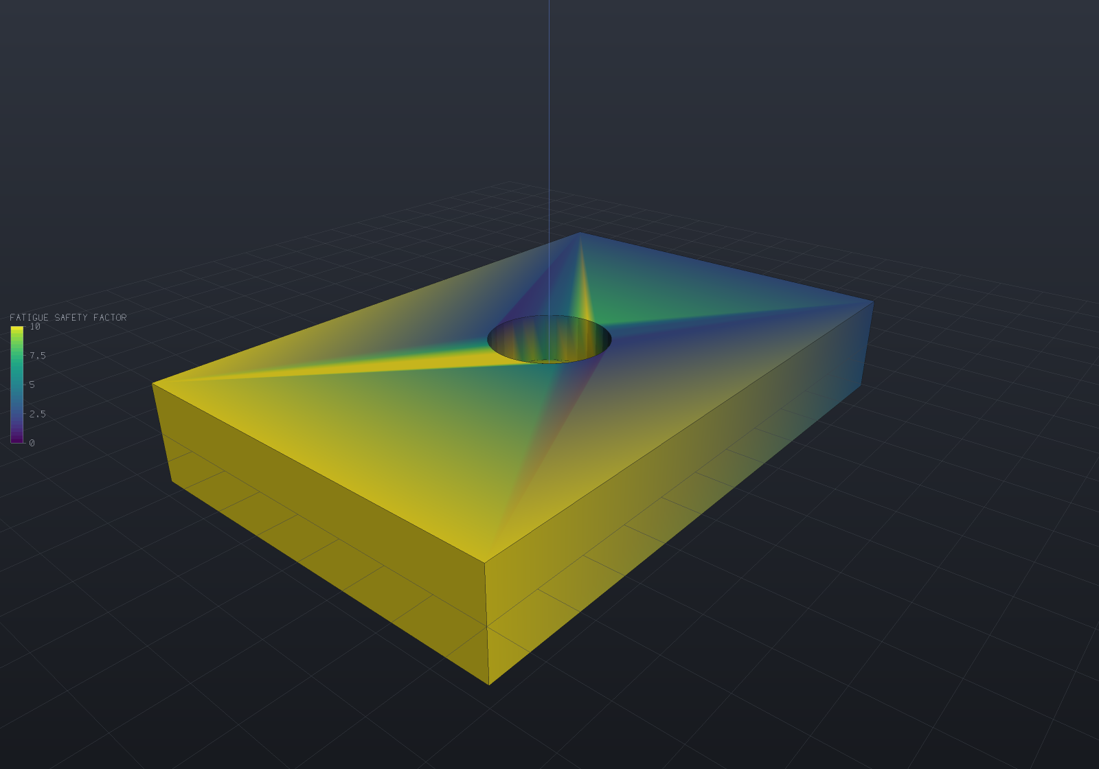

This example runs on the full kernel only — it uses StructuralModel, which the browser build does not ship.

The load cycles between 1800 N downward and 600 N upward. Dark is close to failure: the factors fall toward the built-in end, where the bending stress peaks, and dip around the pocket — the stress concentration — while the lightly stressed free end saturates the top of the band.

[!NOTE] The mesh is coarse on purpose so this page builds quickly, and a coarse mesh understates a concentration’s stress — which overstates its fatigue life. Real fatigue numbers need the peak stress converged (see the error estimate on the structural page), and life is brutally sensitive: with a Basquin slope near −0.1, a 2% stress error is roughly a 24% life error.

The loading model: two cases, proportional

FatigueAnalysis.Evaluate(a, b, curve) takes the two extremes of one proportional load history — the assumption under which every stress component scales together, so one scalar per node captures the cycle. The pair is what StructuralSolver.SolveAll returns from one assembly and one factorization; results solved on different meshes, or answering with different stress-recovery settings, are refused by name (differencing a Direct field against a Superconvergent one would book the recovery gap as alternating stress).

The scalar is the signed von Mises equivalent: the von Mises magnitude carrying the sign of the hydrostatic trace, so a fully reversed load reads R = −1 rather than a pulsating magnitude. The convention is recorded with its reasons: the common alternative (the sign of the absolutely largest principal stress) needs an eigensolve and jumps when two nearly equal principals of opposite sign swap magnitude, while the trace is linear in the stress components — and in the uniaxial state the S-N data was measured in, the two agree exactly.

Per node, with s₁/s₂ the signed equivalents under the two cases:

Quantity	Definition
alternating stress σ_a	(max(s₁,s₂) − min(s₁,s₂)) / 2
mean stress σ_m	(max(s₁,s₂) + min(s₁,s₂)) / 2 (signed; negative is compressive)

The max and min are taken per node, so which case is “worse” may differ across the part, and the case order never matters (asserted as bits).

The S-N catalogue

SnCurve is the Basquin line σ_a = σ'_f·(2N)^b — the amplitude a fully reversed uniaxial test survives for N cycles — plus the ultimate strength the mean-stress corrections anchor on. FatigueMaterials transcribes a handful of rows from the SAE J1099 / Dowling compilations, flagged verify-against-datasheet exactly as StandardHoles’ Trisert table and SheetMaterials’ K-factors are: fatigue constants are fitted to particular material batches, heat treatments and polished laboratory specimens, published sources genuinely disagree, and the authority is the datasheet for your material condition, not this file.

Curve	σ’_f (MPa)	b	S_ut (MPa)	endurance
Steel1015 (SAE 1015 normalized)	827	−0.11	415	168 MPa at 10⁶
Steel1045 (SAE 1045 HR)	948	−0.092	621	250 MPa at 10⁶
Steel4340 (AISI 4340 QT)	1758	−0.0977	1241	426 MPa at 10⁶
Aluminium2024T351	927	−0.113	469	—
Aluminium6061T6	535	−0.102	310	—
Aluminium7075T6	1466	−0.143	578	—

Two decisions carry the table. The endurance limit is DERIVED, never stored beside the line — a steel’s limit is the Basquin line evaluated at its own 10⁶-cycle knee, so the two cannot drift (the same one-source-of-truth rule that keeps the fine-pitch thread table from carrying a tap-drill column), and beyond the knee the curve is flat at that value. And the aluminium rows carry no endurance limit because the material has none — steels arrest small cracks below a threshold stress, face-centred-cubic aluminium does not — a real metallurgical distinction the API keeps rather than smoothing over: below its limit a steel node lives forever, while an aluminium node always has a finite life and a safety factor for it needs a stated design life.

The constants are stored in the form a human can check — MPa, which is both the datasheet unit and the model unit (ModelUnits), so unlike the density lesson there is no conversion for a transcription test to hide behind. Basquin is a high-cycle model: below roughly 10³ cycles plastic strain dominates and the numbers are extrapolations that should be read as “fails fast”, not as a schedule.

Mean-stress corrections

A tensile mean stress shortens life at the same amplitude. The correction folds the cycle onto the R = −1 curve as an equivalent fully reversed amplitude, selectable per run:

MeanStressCorrection	Equivalent amplitude (σ_m > 0)	Character
Goodman (default)	σ_a / (1 − σ_m/S_ut)	Linear line to S_ut — conservative for ductile metals
Gerber	σ_a / (1 − (σ_m/S_ut)²)	Parabola — tracks test data closer, less conservative
None	σ_a	Only right for a genuinely reversed history

Three behaviours are structural and pinned by test: at zero mean both corrections are the identity exactly; at a mean of exactly S_ut the allowable alternating stress is exactly zero (both lines meet the axis there); and a compressive mean takes no benefit by default — compression genuinely retards crack growth, but crediting it requires confidence the mean stays compressive over the whole service life at the surface where cracks start (residual-stress relaxation alone can void it), so the amplitude passes through unchanged on the compressive side, which is what every standard tool defaults to. A mean at or beyond S_ut has failed statically, not in fatigue, and is reported as the life floor below.

Life, the safety factor, and their spellings

// A bar under a fully reversed +/-300 MPa axial load, end to end: two solves, the
// decomposition, the (identity) correction, the life - against the Basquin inversion
// worked by hand: N = 0.5*(300/948)^(1/-0.092) = 1.35e5 cycles, log10 = 5.1303.
// nu = 0 makes the uniaxial state EXACT in the element space, so the check is tight.
var bar = new Part("bar", Shape.Box(40, 10, 10));
var tets = TetMesher.Mesh(bar.GetMesh(),
    new TetMeshOptions { RefineQuality = true, MaxElementSize = 4 });
var mesh = AnalysisMesh.Of(tets);

StructuralModel Case(double sigma)
{
    var model = new StructuralModel(mesh, new Material("steel (nu 0)", 210_000, 0.0));
    model.Fix(Facets.OnPlane(new Vector3d(-20, 0, 0), Vector3d.UnitX));
    model.Traction(Facets.OnPlane(new Vector3d(20, 0, 0), Vector3d.UnitX),
        new Vector3d(sigma, 0, 0));
    return model;
}
var cases = StructuralSolver.SolveAll([Case(300), Case(-300)]);
var fatigue = FatigueAnalysis.Evaluate(cases[0], cases[1], FatigueMaterials.Steel1045);

if (Math.Abs(fatigue.MinLog10Life - 5.1303) > 0.001)
    throw new Exception($"log10 life {fatigue.MinLog10Life} vs the hand-computed 5.1303");
if (fatigue.MinSafetyFactor >= 1)
    throw new Exception("300 MPa is above the 250 MPa endurance limit - the factor must fail");

Four fields publish per node (FatigueResults.Fields() / SampleOnto(displayMesh)), each with a deliberate spelling:

• Fatigue safety factor (dimensionless) — the load multiplier to the mean-stress line: scale the whole history by this factor and the node sits exactly on the line, which is also how the tests verify it (re-solve with the loads scaled by the measured factor; the minimum reads 1.0). Against the endurance limit by default; a material with no endurance limit requires FatigueOptions.DesignLife, refused by name, because a safety factor against infinite life does not exist for it. A node with zero amplitude and no tensile mean has no fatigue mechanism at all and reads NaN — the no-value spelling — rather than an infinity that would poison the legend.
• Fatigue life as log10(cycles) — published as the logarithm because lives spread over many decades and the colour pipeline’s range mapping is linear, so raw cycles would spend the whole legend on the longest-lived node. The units string declares the transform, and the legend reads that declaration: a field whose units say log10(…) gets tick labels in the anti-logged values (1E+05, not 5.1), decade tick placement where the range spans at least two decades, and a title in the base units — see the plot below. Infinite life is NaN — at or below the endurance limit, or zero amplitude — the same “no value” convention the VTU writer uses, which the ranging machinery already skips, so a part that mostly lives forever still gets a usable legend over the nodes that do not. A life below one cycle (including the static-failure branch, mean ≥ S_ut) is floored at 1, i.e. log10 = 0: ranging skips only NaN, so a −∞ would poison the minimum, and sub-cycle “lives” are outside Basquin’s validity anyway.
• Alternating stress and Mean stress (MPa) — the decomposition itself, published so the inputs to the correction are inspectable beside its output.

A life plot, on a log legend

// The same bracket and duty cycle in 6061-T6 aluminium, coloured by LIFE. Aluminium
// here because it has no endurance limit, so EVERY node carries a finite life and
// the whole ramp is populated (the steel plot below shows the other case). The life
// field publishes log10(cycles) and SAYS so in its units string, which is the
// declaration the legend reads: ticks sit on the integer decades and print the
// cycle counts.
var bracket = Shape.Box(60, 40, 10)
    .Subtract(Shape.Cylinder(6, 40).Translate(0, 0, 20));
var part = new Part("bracket", bracket);

var surface = part.GetMesh();
var tets = TetMesher.Mesh(surface, new TetMeshOptions
{
    RefineQuality = true,
    MaxElementSize = 14,
});
var mesh = AnalysisMesh.Quadratic(tets);

StructuralModel Case(double load)
{
    var model = new StructuralModel(mesh, Materials.Aluminium6061);
    model.Fix(Facets.OnPlane(new Vector3d(-30, 0, 0), Vector3d.UnitX));
    model.Force(Facets.OnPlane(new Vector3d(30, 0, 0), Vector3d.UnitX),
        new Vector3d(0, 0, load));
    return model;
}
var cases = StructuralSolver.SolveAll([Case(-1800), Case(600)]);

// A no-endurance-limit material has no infinite-life strength for the safety factor
// to measure against, so a design life is REQUIRED (refused by name without one).
var fatigue = FatigueAnalysis.Evaluate(cases[0], cases[1],
    FatigueMaterials.Aluminium6061T6, new FatigueOptions { DesignLife = 1e7 });

foreach (var field in fatigue.SampleOnto(surface))
    part.AddResult(field);
part.FieldDisplay = new FieldDisplay
{
    Field = FatigueResults.FieldNames.Life,
    // The actionable decades. Lightly stressed nodes carry astronomic lives; an
    // explicit range keeps the legend on the band a decision would read, and the
    // top colour honestly means "10^10 or more".
    Range = new FieldRange(2, 10),
};

var scene = new Scene();
scene.Add(part);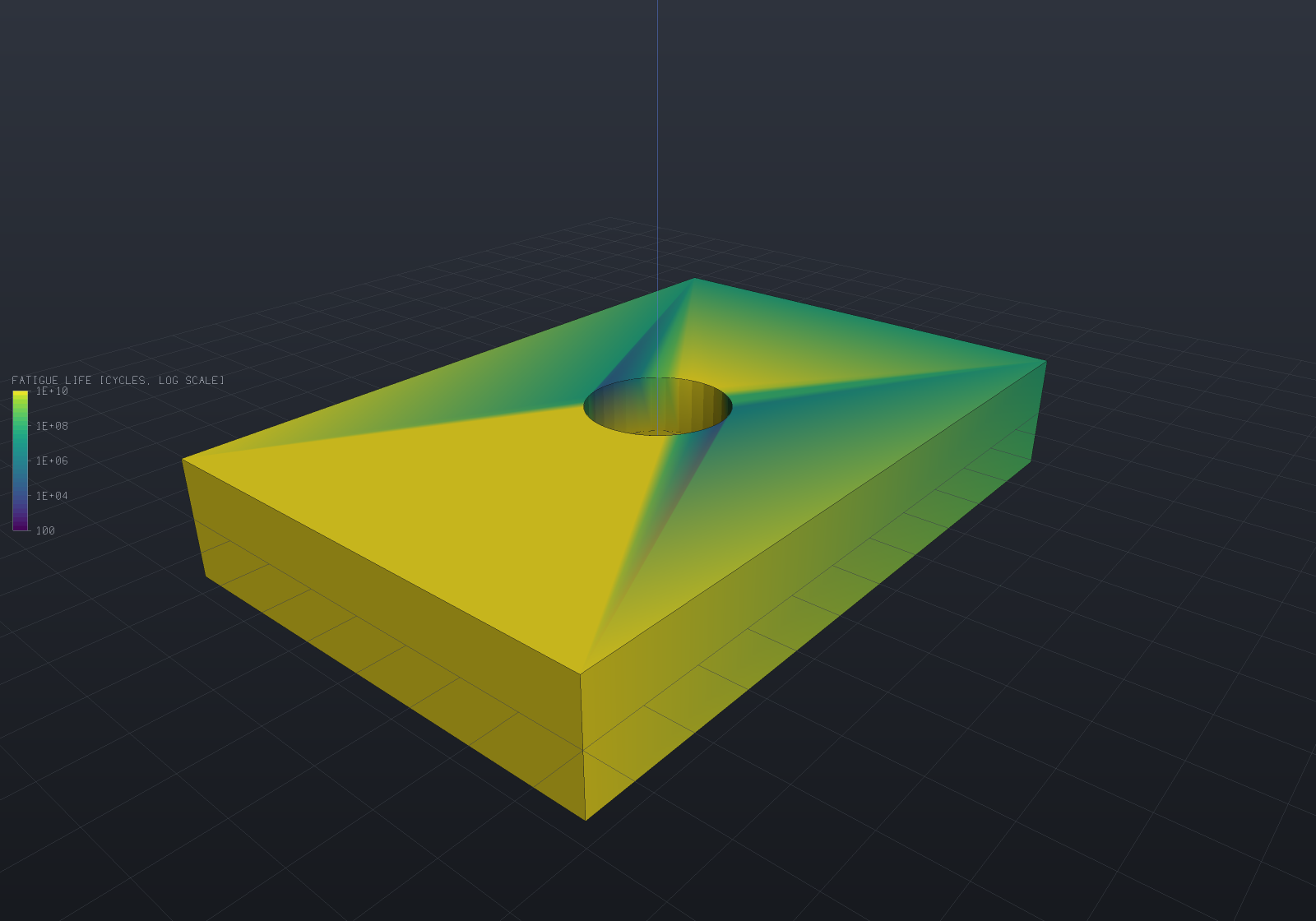

This example runs on the full kernel only — it uses StructuralModel, which the browser build does not ship.

The legend’s ticks sit on the integer decades — 100 through 1E+10 — because the field’s units string is log10(cycles): the declaration is the opt-in, made once by the producer, and the legend renders what it says rather than printing raw logarithms. The colour mapping itself stays linear over the log values, which is exactly what a log-scale colour axis means; a decade tick sits at the linear position of its logarithm, which is where its colour is. Where a log field’s range spans less than two decades the even five-tick layout stays (an interval that short may hold as few as no interior decades — too few ticks to describe a range), still labelled with anti-logged values; and the two end ticks always print the true range, whatever the decades do — a legend that hides its endpoints lies about its range. A field carrying raw decade-spanning values takes the complementary spelling, FieldDisplay.LogScale (see the fields page), which logs the colours instead of the values and prints the same decade ticks.

Infinite life reads as NO VALUE, not as the shortest life

The same bracket in steel shows the other case. A steel node stressed below its endurance limit lives forever — its life is NaN, the “no value” convention the VTU export already uses — and an infinite-life node must not paint the colour of the shortest-lived one, which is what falling to the bottom of the ramp would mean. A no-value node paints a distinct neutral grey (ColorMaps.NoValueColor), and the legend earns a matching NO VALUE swatch below the bar exactly when the displayed field carries one, so most of this part reads honestly as “outlasts any design life” while the stressed region around the bore keeps the colour ramp:

// The bracket in SAE 1045 steel under a 3x duty cycle: the endurance limit makes
// most nodes immortal (life = NaN), which paints the no-value grey with a NO VALUE
// legend swatch — only the stressed region around the bore carries a finite,
// coloured life.
var bracket = Shape.Box(60, 40, 10)
    .Subtract(Shape.Cylinder(6, 40).Translate(0, 0, 20));
var part = new Part("bracket", bracket);

var surface = part.GetMesh();
var tets = TetMesher.Mesh(surface, new TetMeshOptions
{
    RefineQuality = true,
    MaxElementSize = 14,
});
var mesh = AnalysisMesh.Quadratic(tets);

StructuralModel Case(double load)
{
    var model = new StructuralModel(mesh, Materials.Steel);
    model.Fix(Facets.OnPlane(new Vector3d(-30, 0, 0), Vector3d.UnitX));
    model.Force(Facets.OnPlane(new Vector3d(30, 0, 0), Vector3d.UnitX),
        new Vector3d(0, 0, load));
    return model;
}
var cases = StructuralSolver.SolveAll([Case(-5400), Case(1800)]);

var fatigue = FatigueAnalysis.Evaluate(cases[0], cases[1], FatigueMaterials.Steel1045);

foreach (var field in fatigue.SampleOnto(surface))
    part.AddResult(field);
part.FieldDisplay = new FieldDisplay
{
    Field = FatigueResults.FieldNames.Life,
    Range = new FieldRange(2, 10),
};

// The figure's own claim, verified: BOTH populations must exist, or the picture
// shows nothing (all grey is the wrong load; all coloured is the wrong material).
var life = part.Result(FatigueResults.FieldNames.Life)!;
int finite = 0, infinite = 0;
for (int i = 0; i < life.Count; i++)
    if (double.IsNaN(life.ScalarAt(i))) infinite++; else finite++;
if (finite == 0 || infinite == 0)
    throw new Exception($"need both populations: {finite} finite, {infinite} infinite");

var scene = new Scene();
scene.Add(part);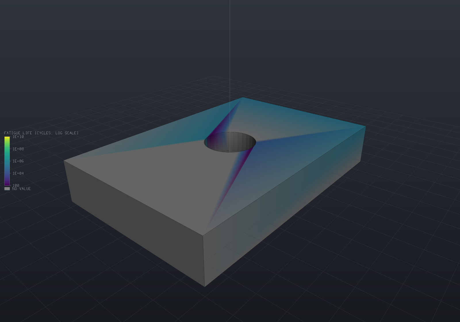

This example runs on the full kernel only — it uses StructuralModel, which the browser build does not ship.

What this deliberately is not

Named rather than approximated, the discipline’s own boundaries:

• Welds. A welded joint’s life is governed by its detail class and geometric (hot-spot) stress, not by the parent metal’s Basquin line — the IIW / Eurocode nominal-stress and hot-spot methods are their own discipline, and running this over a weld answers the wrong question.
• Multiaxial criteria beyond von Mises equivalence. Non-proportional load paths rotate the principal frame and need critical-plane methods (Findley, Fatemi–Socie) — a different computation over a different input. The structural tell lives inside the signed von Mises itself: a reversed pure shear cycle is invisible to any scalar signed equivalent, because negating a pure shear tensor is a rotation of it — no invariant can tell the two halves apart. That is precisely the case critical-plane methods exist for.
• Surface and size effects applied silently. The catalogue’s constants are polished-specimen values and stay that way; WithFactors (below) is how a real part’s surface, size and reliability knock the endurance end down — a derivation the caller asks for, never a default.

Marin factors: the corrected curve is derived, the row stays pristine

The catalogue rows are polished-specimen fits, which makes them upper bounds for any real part. SnCurve.WithFactors(surface, diameter, reliability) derives a corrected curve from the classical Marin correlations — MarinFactors.Surface (the a·S_ut^b finish rows), MarinFactors.Size (the rotating-bending diameter effect; omit the diameter for axial loading, which has none) and MarinFactors.Reliability (the tabulated 8%-scatter shifts) — without the transcribed row ever being edited, the same derived-vs-stored rule the endurance limit itself follows.

var pristine = FatigueMaterials.Steel1045;
var machined = pristine.WithFactors(
    SurfaceFinish.Machined, diameterMm: 25, reliability: 0.99);

Console.WriteLine(pristine);
Console.WriteLine(machined);

// The construction pivots at 10^3 cycles (where plastic strain dominates and the
// factors classically do not apply) and scales the endurance end exactly.
if (Math.Abs(machined.StressAt(1e3) - pristine.StressAt(1e3)) > 1e-9 * pristine.StressAt(1e3))
    throw new Exception("the 10^3-cycle pivot must be unchanged");
if (machined.EnduranceLimit! >= pristine.EnduranceLimit!)
    throw new Exception("the corrected endurance must fall");

The factors multiply the endurance limit, not σ’_f: surface finish, size and scatter govern crack initiation, which dominates at long life, so the corrected line passes through the pristine line’s own 10³-cycle point (Basquin’s validity floor) and through k·S_e at the unchanged knee — Shigley’s two-anchor construction with the curve’s own low-cycle value as the anchor rather than a second transcribed constant. The ultimate strength is untouched (a finish does not change a static failure), a factor of exactly 1 returns the pristine curve verbatim, and the correlations refuse what they cannot answer by name: a knee at or below the pivot, diameters past the 254 mm data, and reliabilities off the standard table (interpolating a quantile through it would invent precision the 8%-scatter assumption does not have). The correlations themselves are transcribed verify-against-datasheet like every constant table here — the classic worked values (machined at 690 MPa → 0.798, 32 mm → 0.858, 99% → 0.814) are the transcription tests.

For aluminium the reference life must be stated. A knee-less line falls forever, so there is no endurance knee for WithFactors to anchor on — use WithFactorsAt(finish, referenceLife, …) (or WithEnduranceFactorAt(factor, referenceLife)), which knocks the strength down AT that life (5e8 cycles is the rotating-beam convention) and re-fits through the same 10³ pivot, leaving the line knee-less. The reference life is required rather than defaulted because it is the claim being made.

Variable amplitude: rainflow over a transient run

Two static cases cannot carry a time history; a transient solve’s stored states can, and are exactly what the rainflow overload consumes. Rainflow.Count is ASTM E1049’s own three-point algorithm — the standard’s worked example is transcribed as a test, cycle for cycle — and FatigueAnalysis.Evaluate(transient, curve, rainflowOptions) runs it over every node’s signed von Mises history with Miner’s-rule damage accumulation, the mean-stress correction applied per counted cycle through the same EquivalentAlternating the static path uses.

// The ASTM E1049 worked example: seven counts, one of them the full cycle E-F.
double[] series = [-2, 1, -3, 5, -1, 3, -4, 4, -2];
foreach (var cycle in Rainflow.Count(series))
    Console.WriteLine(cycle);

// The pipeline: an irregular load history no static pair can carry, counted per node.
var tets = TetMesher.Mesh(
    new Part("bar", Shape.Box(40, 10, 10)).GetMesh(),
    new TetMeshOptions { RefineQuality = true, MaxElementSize = 10 });
var model = new StructuralModel(AnalysisMesh.Of(tets), Materials.Steel);
model.Fix(Facets.OnPlane(new Vector3d(-20, 0, 0), Vector3d.UnitX));
model.Force(Facets.OnPlane(new Vector3d(20, 0, 0), Vector3d.UnitX), new Vector3d(30000, 0, 0));

var run = TransientSolver.Solve(model, new TransientSolveOptions(2e-5, 120)
{
    LoadFactor = t => Math.Sin(90000.0 * t) + 0.4 * Math.Sin(23000.0 * t),
});

var fatigue = FatigueAnalysis.Evaluate(run, FatigueMaterials.Steel1045);
Console.WriteLine(fatigue);
if (fatigue.MaxDamage <= 0)
    throw new Exception("an over-endurance swing must accumulate damage somewhere");

What the counting sees is the stored states: a reversal that fell between stored steps was never sampled and is never counted, so a run that feeds fatigue should store every step (StoreEvery = 1, the default). The per-node series costs one scalar per stored state — small beside the full fields each state already retains — which is why the extraction runs at every node rather than at preselected hot spots: the “which node is worst” answer is the point of the field.

The open end of the history is an option, because ASTM E1049 names two honest readings. By default the history is one-shot — a load event with a beginning and an end, which is what a transient run is — and the residual ranges the counting cannot close are the standard’s half cycles. AssumeRepeating = true reads it as one period of a repeating load: the series is rearranged to begin at its largest-magnitude extremum (E1049’s own prescription, under which every count closes) and the residual halves pair into full cycles, so a block program counted per block accumulates no phantom boundary halves. The two modes agree on damage for a constant-amplitude history; what changes is the cycle structure reported.

The answer publishes as three fields: Fatigue damage — Miner damage per pass of the stored history, the quantity that composes (k passes accumulate k·damage; life is 1/damage repetitions) — Fatigue repetitions as log10(repetitions), with the static path’s spellings (NaN = no damage anywhere = infinite life; the one-repetition floor covers the static-failure branch) — and Fatigue load factor, the spectrum’s safety factor, below. The names differ from the static pair’s on purpose: a part carrying both analyses would otherwise have one silently replace the other (same name replaces, by design), and they answer different questions over different inputs.

The spectrum safety factor

RainflowFatigueResults.SafetyFactor (and FatigueAnalysis.LoadFactor for a spectrum from anywhere else) is the multiplier on the whole load history at which the counted spectrum reaches its damage target — the same claim the static pair’s radial factor makes, and verified the same way: scale the loads by it, re-solve, re-count, and the damage lands on the target.

Two targets, exactly as the static path has two:

RainflowFatigueOptions.DesignRepetitions	The factor measures against
null (default)	infinite life — the multiplier at which the worst counted cycle first reaches the endurance limit and damage first appears
R	a Miner damage of 1/R — the multiplier at which one pass in R exhausts the part

// A load spectrum with several distinct amplitudes and a tensile mean - the case no
// single (amplitude, mean) pair describes.
RainflowCycle[] spectrum =
[
    new(Range: 500, Mean: 120, Count: 1),     // amplitude 250
    new(Range: 320, Mean:  90, Count: 8),     // amplitude 160
    new(Range: 180, Mean:  60, Count: 40),    // amplitude 90
];
var curve = FatigueMaterials.Steel1045;

// Against infinite life: closed form, because each cycle reaches the endurance limit at
// its OWN static radial factor and the spectrum reaches it at the smallest of them.
double forever = FatigueAnalysis.LoadFactor(spectrum, curve);
Console.WriteLine($"to infinite life: x{forever:F4}");

// Against a stated life: the root of D(k) = 1/R, bracketed.
double toTenThousand = FatigueAnalysis.LoadFactor(
    spectrum, curve, MeanStressCorrection.Goodman, designRepetitions: 1e4);
Console.WriteLine($"to 1e4 repetitions: x{toTenThousand:F4}");

// The oracle is the definition: scale every cycle by the factor and the damage IS the
// target. (Scaling the cycles is what scaling the loads does, the stress being linear.)
RainflowCycle[] scaled =
    [.. spectrum.Select(c => new RainflowCycle(
        toTenThousand * c.Range, toTenThousand * c.Mean, c.Count))];
double damage = FatigueAnalysis.Damage(scaled, curve);
if (Math.Abs(damage - 1e-4) > 1e-10)
    throw new Exception($"damage {damage} vs the 1e-4 target");

Is there a closed form? Partly, and the boundary is worth stating because it is where a plausible shortcut goes wrong. Damage is a sum of power-law terms, so if every cycle’s equivalent amplitude were linear in the multiplier the whole sum would scale as k^(−1/b) and the answer would be exactly (R·D)^b for the damage D at unit load — one line of algebra. Two ordinary things break that linearity:

• The endurance knee. Cycles join the sum as the multiplier grows, so the coefficient is piecewise and a closed form read off the unit-load damage overstates the factor (measured 4.5% on a two-level spectrum whose smaller cycles cross).
• A tensile mean under a correction. The equivalent amplitude is k·σ_a / (1 − k·σ_m/S_ut), which is not a power of k at all — and it diverges at k = S_ut/σ_m, a hard static-failure ceiling the factor can never reach. The closed form understates there (measured 12.9%).

So there is one bracketed solve for every case rather than a closed form with conditions, and the closed form is kept where it belongs — as the test oracle, on the two spectra where it is exact (a knee-less curve, and a steel spectrum entirely above its knee at both ends), where it agrees with the solve to within an ulp or two. The infinite-life target is the one case that is closed form throughout, because “the multiplier at which damage first appears” is per-cycle rather than accumulated: it is the static radial factor of each cycle against the endurance limit, minimum over the spectrum — the same helper the static pair’s field is built from, so a one-cycle spectrum answers bit-identically.

[!NOTE] The endurance knee puts a genuine step in the damage function: a cycle crossing it goes from contributing nothing to contributing count/10⁶, so D(k) = target has no solution when the target lands inside a step. The factor reported is then the crossing itself — the smallest multiplier at which the target is reached — and that step is the flat-line S-N model’s own artefact, not this solve’s. The standard remedy is SnCurve.WithHaibachSlope() — continue the line past the knee at the shallower slope b' = b/(2 + b), so a sub-limit cycle carries a small finite damage and D(k) becomes continuous (a target inside the old step then has a solution). It removes the endurance plateau, so the resulting curve has no infinite-life strength and DesignRepetitions becomes required — the same rule aluminium earns.

A material with no endurance limit has no infinite life to measure against, so there DesignRepetitions is required and its absence is refused by name — verbatim the static path’s rule for FatigueOptions.DesignLife, for verbatim its reason. And a node whose history never moves carries no counted cycle, so it reads NaN however large its steady stress: rainflow measures cycles, and a steady load is a static-strength question the static pair answers instead (two identical cases report the S_ut/σ_m margin).

[!WARNING] That NaN has two causes and only one of them is honest, and the second is the reversed pure shear above arriving through the spectrum: negating a pure shear tensor is a rotation of it, so both halves of the cycle read the same signed von Mises and the series is constant — indistinguishable, here, from a node that genuinely never moves. So a NaN factor means “this node’s history carries no cycle in the scalar equivalent”, which is the reading a truly static node deserves and an over-estimate for a node cycling in shear. The factor inherits the scalar’s blind spot exactly as the damage does — it does not add one, and it does not repair one; critical-plane methods are where that case is answered.

Cost follows the target, which is why they are priced separately: on a 135-node mesh with 241 stored states and up to 93 counted cycles per node (win-x64, Release), the whole evaluation takes 3.5 ms against the infinite-life target and 18.2 ms (5.2×) against a stated one — the counting is the shared floor, the closed form is one more pass over cycles that already exist, and the bracketed solve is about sixty damage evaluations per node.

Verification

From the test suite (FatigueTests, SnCurveTests), on the bar whose uniaxial state is exact in the element space (ν = 0, the same trick the multi-material bar uses):

Check	Measured
σ_a/σ_m from two load cases vs an oracle re-derived from the displacement solution	40 / 60 MPa, ≤ 1e-10 relative at every node
equal-and-opposite loads read R = −1	mean ≤ 1e-13 of the amplitude (measures exactly 0: negation commutes with IEEE rounding bit for bit)
the line at one reversal is σ’_f	bit-exact (Math.Pow(1, b) is 1)
the endurance knee is on the line, and the curve is flat beyond it	bit-exact
SAE 1045 endurance limit vs the hand-worked 948·(2·10⁶)^(−0.092)	249.53 MPa
life/stress inverse round-trip below the knee	≤ 1e-12 relative
Goodman and Gerber at zero mean	identity, bit-exact
allowable amplitude at σ_m = S_ut	exactly zero, both lines
loads scaled by the measured safety factor	the critical node lands ON the line: min factor 1.0 to 1e-9
R = −1 at 400 MPa, full pipeline, vs the hand-computed life	5.92e3 cycles, log10 within 1e-6 of the Basquin inversion
steel endurance limits vs their ultimate strengths	0.40 / 0.40 / 0.34 — near the classical one-half correlation, inside the asserted 0.30–0.55 band a mistyped exponent cannot survive
ASTM E1049 Fig. 6 worked example (RainflowTests)	all seven counts reproduced — range, mean AND half/full status, in algorithm order
rainflow decomposes the total variation, sum(2·count·range) vs the turning points’ own `sum	Δ
a constant-amplitude history (transient states alternating between the SolveAll pair) vs the static-pair answer	the counted cycle’s amplitude and mean bit-equal the static decomposition; damage exactly count/life
the spectrum load factor applied: re-solve the whole history with the loads scaled by it	the critical node’s damage lands on the target — 1.0000e-4 against 1e-4, min factor 1.0 to 1e-9, Goodman AND Gerber
the closed form (R·D)^b where the spectrum is a pure power law (knee-less curve; steel spectrum above its knee)	1.0329781076872908 vs 1.0329781076872908 (bit-equal) and 1.1561344804722387 vs …89 (2 ulp)
…and where it is not	overstates by 4.5% across the endurance knee, understates by 12.9% under a tensile mean — the solved factor lands on the target in both
a ONE-cycle spectrum vs the static radial factor at the same life (a bisection over a Miner sum against a line intersection)	agree to ≤ 1e-9 relative at every mean −100…400 MPa, all three corrections, both above and below a factor of 1
a constant-amplitude history’s factor vs the static pair’s	bit-equal against infinite life at every node; 1.1744 both ways against a stated target (two cycles per pass, so R repetitions is a life of 2R cycles)
the infinite-life factor as a threshold	damage exactly 0 a nanometre under it and count/10⁶ a nanometre over — the flat line’s own step
the factor is inverse in the load scale	a history scaled by 1.01 reports 1/1.01 to 1e-9