Buckling, damping and frequency response

A slender part under compression can fail long before its material yields: it goes unstable and folds sideways. EngrCAD.Fea finds the load at which that happens with a linear buckling analysis on the same tetrahedral meshes the mesher produces, with the same materials and the same supports the structural and modal solvers already take. The eigenproblem is

(K + lambda·Kg) phi = 0

where Kg is the geometric stiffness the prestress from a prior static solve produces, and lambda is the multiple of that load case at which the structure loses stability.

var part = new Part("strut", Shape.Box(100, 10, 10));

var surface = part.GetMesh();
var tets = TetMesher.Mesh(surface, new TetMeshOptions
{
    RefineQuality = true,
    MaxElementSize = 14,     // deliberately coarse - this page is a picture, not a study
});

// QUADRATIC elements, and it matters more here than anywhere else: a buckling load is a
// ratio of a bending stiffness to a geometric softening, so linear tetrahedra's bending
// over-stiffness enters the answer undiluted. See "Use quadratic elements" below.
var model = new StructuralModel(AnalysisMesh.Quadratic(tets), Materials.Steel);
model.Fix(Facets.OnPlane(new Vector3d(-50, 0, 0), Vector3d.UnitX));
model.Force(Facets.OnPlane(new Vector3d(50, 0, 0), Vector3d.UnitX), new Vector3d(-1000, 0, 0));

var statics = StructuralSolver.Solve(model);                  // the prestress
var buckling = BucklingSolver.Solve(statics, new BucklingSolveOptions { ModeCount = 1 });

// The factor multiplies the WHOLE load case, so the critical load is 1000 N times it.
foreach (var field in buckling.SampleOnto(surface))
    part.AddResult(field);
part.FieldDisplay = new FieldDisplay
{
    Field = BucklingResults.FieldNames.Shape(1),
    Deform = BucklingResults.FieldNames.Shape(1),
    DeformScale = 12,
};

var scene = new Scene();
scene.Add(part);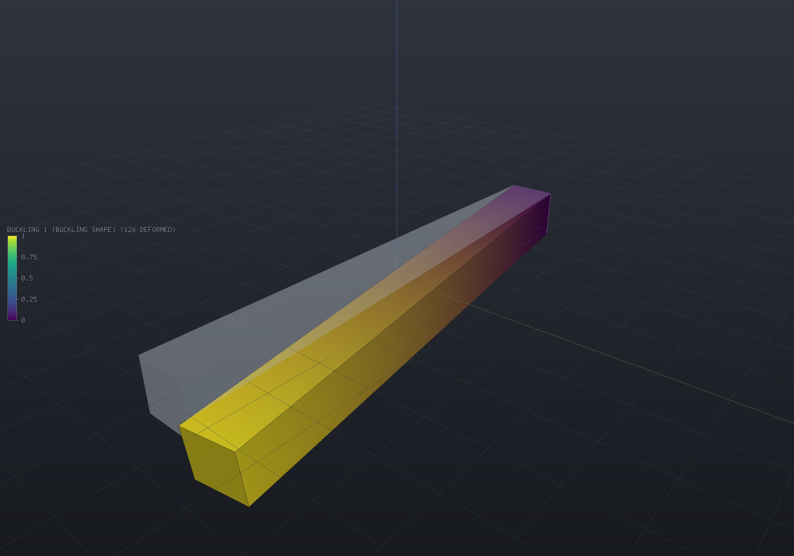

A cantilever strut in its first buckling mode — This example runs on the full kernel only — it uses TetMesher, which the browser build does not ship.

A 100 × 10 × 10 steel strut built in at one end and pushed axially at the free one, shown in its first buckling mode with the unloaded shape ghosted behind: 738 elements, 4 524 degrees of freedom, and a critical load factor of 43.454 — so a 1 000 N reference load means the strut buckles at 43 454 N. Euler’s pi²EI/(2L)² for this fixed–free case is 43 180 N and the shear-corrected value is 42 904 N, so this deliberately coarse mesh is 1.28% above the truth, from above, which is where a Rayleigh quotient over a finite element subspace has to be.

The load factor multiplies the load CASE, not a number in it

A linear static solve’s stress field is homogeneous of degree one in every load it was given — forces, pressures, tractions, gravity, a thermal field, an enforced displacement — so the geometric stiffness scales with all of them together and the eigenvalue is a factor on the case as a whole.

Nothing in the API is called “the critical load”, deliberately. A strut pushed from both ends has an applied resultant of exactly zero while its stress field is precisely what buckles it, so a scalar critical load would either read zero or would have to guess which half of the load case was meant. Multiply your own reference load by the factor:

double margin = buckling.CriticalLoadFactor;        // > 1 is stable, with that much margin
double criticalLoad = margin * appliedLoad;         // whatever "the load" means to you

Only positive factors are reported

A negative factor is the multiple at which the reversed load case buckles. That is a real answer to a different question — a bending prestress routinely produces both signs — so the solver returns the positive family in ascending order and stops at the first non-positive value rather than skipping past it. A load case with no positive factor at all (a body entirely in tension is the ordinary example) is refused by name rather than reported as an empty list.

Use quadratic elements

4-node tetrahedra are known to be too stiff in bending, and a buckling load is a ratio of a bending stiffness to a geometric softening — so the over-stiffness enters undiluted instead of being averaged against anything. Measured on a 120 × 6 × 6 pinned-pinned column whose true critical load is 15 468 N:

mesh	linear elements	quadratic elements
8×1×1	171 602 N (+1 009%)	15 554 N (+0.55%)
16×2×2	55 108 N (+256%)	15 450 N (−0.12%)
32×3×3	26 137 N (+69.0%)	15 438 N (−0.20%)
48×4×4	20 402 N (+31.9%)	—

Where the static cantilever’s tip deflection is 14% low at 12 288 linear elements, the same elements put a column’s critical load an order of magnitude high on a coarse mesh, and are still 32% high at 3 550 degrees of freedom where the quadratic answer converged to 0.2% with 414. Use AnalysisMesh.Quadratic for any stability analysis.

Verification: all four Euler end conditions

A 120 × 6 × 6 steel column at slenderness 69.3, 24 × 2 × 2 quadratic elements, Poisson’s ratio exactly zero so the lateral end restraints are satisfied identically and the prestress is exactly -P/A (measured deviation from uniform: 5.45e-13 relative). Against P = pi²EI/(K·L)²:

ends	K	Euler	Engesser	measured	vs Euler	vs Engesser
pinned–pinned	1.0000	15 544.6 N	15 468.3 N	15 440.3 N	−0.671%	−0.181%
fixed–free	2.0000	3 886.2 N	3 881.4 N	3 879.6 N	−0.169%	−0.046%
fixed–pinned	0.6992	31 800.4 N	31 482.6 N	31 338.4 N	−1.453%	−0.458%
fixed–fixed	0.5000	62 178.5 N	60 974.9 N	60 550.5 N	−2.618%	−0.696%

Euler’s derivation has no shear deformation and a three-dimensional solid has it, so the measured load converges below the Euler value by Engesser’s ratio 1/(1 + P_E/(kAG)) — the buckling twin of the Timoshenko correction the modal page quotes. That is why the fixed–fixed row, whose Euler load is four times larger and whose shear correction is therefore four times bigger, is the furthest from Euler and no further from the truth.

Refinement is monotone from above — 16 122.23 / 15 553.67 / 15 449.65 / 15 438.52 N at 4 / 8 / 16 / 32 elements along the length — which is a theorem rather than a property of the fixture: the discrete factor is a Rayleigh quotient minimised over the element subspace, and a coarser mesh is a smaller subspace.

The buckled shape is the half sine to 2.4e-6 over 49 centroidal nodes, and doubling the reference load halves the factor so their product is unchanged to 0.00e0 relative — the cheapest possible check that the geometric stiffness is linear in the prestress.

Stress stiffening: the frequencies of a preloaded part

The same geometric stiffness answers a second question. A guitar string, a spinning blade and a preloaded bolted joint all ring at frequencies their preload sets, and ModalSolveOptions.Prestress adds Kg to the modal problem:

var statics = StructuralSolver.Solve(loadedModel);        // the preload case
var results = ModalSolver.Solve(model, new ModalSolveOptions
{
    ModeCount = 3,
    Prestress = statics,
    PrestressScale = 0.5,                                 // half the reference load
});

PrestressScale multiplies the stress field without re-solving, because a linear solve’s stress is homogeneous of degree one in its loads — so a frequency-versus-load curve is one static solve and N eigen-solves.

Tension raises every frequency and compression lowers them, and the two features meet exactly at the critical load: K + lambda_cr·Kg is singular by definition, its null vector is the buckling shape, and the lowest natural frequency is zero. Past it there is no vibration problem left, and the factorization refuses by name.

The classical law for a pinned-pinned beam is omega²(P)/omega²(0) = 1 + P/P_cr, with P positive in tension. Measured on the discrete three-dimensional column with P_cr taken from the buckling solve, it holds to 7.4e-10 relative across the whole range:

P/P_cr	−1.0	−0.5	0	+0.25	+0.5	+0.9
f (Hz)	1 377.77	1 193.19	974.23	843.71	688.89	308.08
ω²/ω²(0)	2.000000	1.500000	1.000000	0.750000	0.500000	0.100000
relative error	−7.4e-10	−4.1e-10	0	1.9e-10	4.3e-10	6.5e-10

It is that tight because this column’s buckling shape and its first vibration shape are the same half sine, so the ratio of two Rayleigh quotients over one vector is the ratio of their numerators. One table checks the geometric stiffness, the load factor and the stress-stiffened modal path against each other.

Damping

RayleighDamping is C = alpha·M + beta·K, whose point is that the undamped modes still diagonalise it: the equations separate into one scalar oscillator per mode and the damping is a per-mode ratio zeta_n = alpha/(2·omega_n) + beta·omega_n/2.

var damping = RayleighDamping.FromRatios(50, 0.02, 500, 0.02);   // 2% at both ends
double zeta = damping.RatioAtFrequency(180);                     // 1.05% in between

The curve is a U — the mass term falls as 1/omega, the stiffness term rises linearly — so two fitted points pin it everywhere and everything outside the fitted range is damped more than either fitted value. Fitting 3% at 20 Hz and 1% at 800 Hz gives 11.5% at 5 Hz and 6.2% at 5 kHz, which is how a high mode nobody looked at comes to be nearly over-damped. HarmonicResponse.DampingRatios reports the ratio used for every mode for exactly that reason, and a fit with no solution (a ratio falling faster than 1/omega) is refused rather than returned with a negative coefficient — negative damping adds energy.

What proportional damping does not cover, stated rather than implied away. It is the special case in which one damping matrix happens to be diagonalised by the undamped real modes. Physical damping usually is not: a discrete dashpot, two materials with different loss factors in one model, viscoelasticity, joint friction and structural (hysteretic) damping all leave phi' C phi with off-diagonal terms — and then the damped system’s modes are no longer the undamped ones. The eigenproblem becomes the quadratic (lambda²M + lambda·C + K) phi = 0, whose eigenvalues and eigenvectors are complex and whose standard solution linearises it into a 2n-dimensional state-space problem in a non-symmetric matrix pair. That is a different solver, not a bigger version of this one, and nothing here attempts it. ModalDamping.Uniform (a flat ratio) and ModalDamping.PerMode (a measured table) are the other two forms, both proportional by construction.

Frequency response

Each mode is a scalar oscillator, so the steady-state response to a harmonic load is a closed form and the whole sweep costs one dot product per mode plus a complex division per (mode, frequency) pair. Nothing is assembled and nothing is factorized.

var tets = TetMesher.Mesh(
    new Part("beam", Shape.Box(80, 12, 8)).GetMesh(),
    new TetMeshOptions { RefineQuality = true, MaxElementSize = 12 });

var model = new StructuralModel(AnalysisMesh.Quadratic(tets), Materials.Steel);
model.Fix(Facets.OnPlane(new Vector3d(-40, 0, 0), Vector3d.UnitX));
model.Force(Facets.OnPlane(new Vector3d(40, 0, 0), Vector3d.UnitX), new Vector3d(0, 0, -50));

var modes = ModalSolver.Solve(model, new ModalSolveOptions { ModeCount = 4 });
var statics = StructuralSolver.Solve(model);            // for the truncation correction

var response = HarmonicSolver.Solve(modes, new HarmonicSolveOptions
{
    Frequencies = HarmonicSweep.Around(modes.Mode(1).Frequency, 0.05, 201),
    Damping = ModalDamping.Rayleigh(
        modes.Mode(1).Frequency, 0.02, modes.Mode(4).Frequency, 0.02),
    StaticCorrection = statics,
});

// The peak of the sweep lands on the first natural frequency.
double peak = response.Frequencies[response.PeakFrequencyIndex];
if (Math.Abs(peak - modes.Mode(1).Frequency) > 0.01 * peak)
    throw new Exception($"the sweep peaked at {peak:N1} Hz, not at {modes.Mode(1).Frequency:N1}");

// And the fitted ratios reach the modes unchanged.
if (Math.Abs(response.DampingRatios[0] - 0.02) > 1e-12)
    throw new Exception($"mode 1 was damped {response.DampingRatios[0]:P4}, not 2%");

Console.WriteLine(response.ToText());

The load comes from the modal model’s own applied forces. Every load type reduces to consistent nodal forces when it is applied, so one model carries the supports, the loads and the modes computed from it, and there is no second place for a load to be specified and forgotten. A thermal load is refused by name — it enters a static solve as an element integral rather than a nodal force, so accepting it would silently drop it — and so is a free-free model, whose rigid modes contribute F_n/(0 - W²) and grow without bound as the frequency falls.

Damping is required rather than defaulted, because a default would be this library inventing a material property. ModalDamping.None is allowed and says so explicitly; an undamped mode driven at exactly its own frequency then returns a non-finite modal coordinate, left alone rather than clamped to a large number nobody chose.

Base (support) excitation — a shaker or seismic input — drives the model through its supports instead of by a nodal force. Set HarmonicSolveOptions.BaseExcitation:

BaseExcitation = new BaseExcitation(new Vector3d(0, 0, 1), BaseMotionKind.Acceleration, 9810),

It needs no new mathematics — in relative coordinates the modal force is exactly -Gamma_d·a_g, the participation factor the modal results already carry. BaseMotionKind says whether the constant amplitude is an acceleration (frequency-independent), a velocity (a_g = omega·v_g) or a displacement (a_g = omega²·u_g, so the modal force scales with the sweep). The response is the relative displacement (HarmonicResponse.IsRelativeToBase), which is the right quantity for stress because a rigid ground motion carries none; the absolute displacement is that plus the rigid ground field. The whole base moves together — independent support-group motion is a per-group static solve, stated as v1’s boundary — and a model that also carries nodal forces, or a base excitation combined with a static correction, is refused by name.

Truncation is a correction, not a caveat

Modal superposition keeps only the modes that were extracted, so it misses the static flexibility of every mode above them. Passing StaticCorrection switches on the mode-acceleration form

u(W) = u_static + sum_n phi_n F_n [1/(w_n² - W² + 2i·zeta·w_n·W) - 1/w_n²]

whose bracket vanishes at W = 0 — so the response is exactly the static answer there however few modes were kept, and the missing modes’ static flexibility is carried at every other frequency. Measured: a one-mode response reproduces the full static tip deflection to 1.8e-16 relative, where the uncorrected one-mode sum is 3.01% short. HarmonicResponse.TruncationError reports what the plain sum would have missed, and is NaN without a static solve — because then it is not small, it is unknown.

Verification against the single-oscillator closed forms

On a tip-driven cantilever:

quantity	closed form	measured
resonant amplification	`1/(2·zeta)` = 25.000	25.006 (0.02%)
half-power bandwidth, zeta = 1%	2.0000%	2.0005%
half-power bandwidth, zeta = 2%	4.0000%	4.0034%
half-power bandwidth, zeta = 5%	10.0000%	10.0541%
phase lag at resonance	90°	90.073°
static limit with the correction	exact	1.8e-16 relative

Two of those numbers have a trap in them. The amplification is measured against that mode’s static contribution, not the structure’s whole static deflection — the other modes supply 3.01% of this cantilever’s static tip, and dividing by the whole thing reads as a 3% solver error that is entirely a mistake in the measurement. And the phase is read at the mode’s own frequency rather than at the sweep’s peak sample: those are two steps apart at this resolution, and detuning by 0.04% of the frequency rotates the phase 1.15° at 2% damping, so probing the peak sample would measure the sweep instead of the response.

The direct per-frequency solve

DirectHarmonicSolver factorizes the full complex system (K - W²M + i·W·C + i·eta·K) at every sweep point over SparseLdlt’s complex symmetric LDLᵀ. Its value is fidelity, not speed — the cost is one complex factorization per frequency, hundreds of times a modal sweep, and nothing amortises across sweep points because the matrix carries the frequency — so reach for it where modal superposition structurally cannot go: non-proportional damping, where phi' C phi has off-diagonal terms and the per-mode scalar oscillators the modal method is made of no longer exist.

That damping lives on the model, not on the solve options, because it is geometry-attached data no per-mode ratio can carry: SetDamping states Rayleigh coefficients model-wide or per region (two regions with different values are already non-proportional), and Dashpot places a discrete viscous damper at a node or between two — whose coupling block can land where the stiffness pattern has no entry at all, the union-pattern case the factorization exists for.

var tets = TetMesher.Mesh(
    new Part("beam", Shape.Box(80, 12, 8)).GetMesh(),
    new TetMeshOptions { RefineQuality = true, MaxElementSize = 12 });

var model = new StructuralModel(AnalysisMesh.Quadratic(tets), Materials.Steel);
model.Fix(Facets.OnPlane(new Vector3d(-40, 0, 0), Vector3d.UnitX));
model.Force(Facets.OnPlane(new Vector3d(40, 0, 0), Vector3d.UnitX), new Vector3d(0, 0, -50));

// Damping on the MODEL: material damping everywhere, plus a discrete damper to ground at
// the tip — the non-proportional combination no per-mode ratio can express.
model.SetDamping(new RayleighDamping(0, 2 * 0.02 / (2 * Math.PI * 900)));
int tip = 0;
for (int v = 0; v < model.Mesh.NodeCount; v++)
    if (model.Mesh.Position(v).X > model.Mesh.Position(tip).X) tip = v;
model.Dashpot(tip, new Vector3d(0, 0, 1), 0.05);

var response = DirectHarmonicSolver.Solve(model, new DirectHarmonicOptions
{
    Frequencies = HarmonicSweep.Logarithmic(50, 5000, 12),
});

if (!response.Report.NonProportional)
    throw new Exception("a dashpot beside material damping is non-proportional");
if (response.Report.WorstRelativeResidual > 1e-7)
    throw new Exception($"backward residual {response.Report.WorstRelativeResidual:E1}");
Console.WriteLine(response.ToText());

Three behaviours are decided rather than discovered. An undamped model is accepted — the response is real and grows without bound toward each resonance, which is the true answer — but driven exactly at a resonance the factorization refuses loudly, naming the physics: an undamped structure at its own natural frequency has no steady state to report. A non-zero prescribed support offset is refused (it is a static answer riding on the oscillation — superpose a static solve; an oscillating support is base excitation, filed). An unrestrained body is accepted: K - W²M is nonsingular at almost every frequency, and the low-frequency answer is the rigid body’s own |u| = F/(W²·m) — verified against exactly that closed form.

The two methods check each other where both apply: on a proportionally damped model the direct solve and the corrected modal sweep agree to 3.5e-6 relative over a six-point sweep bracketing the first resonance (the gap is the modal truncation the correction cannot carry at non-zero frequency), exactly (1e-9) on a model whose one mode is the complete basis, and against a hand-built complex 2x2 oracle for a dashpot coupling two nodes that share no element. The report carries the worst backward residual |Zu - f|/|f| over the sweep — 7.4e-9 measured near resonance, the honest figure for an unpivoted factorization — and the smallest pivot magnitude met, which is the conditioning tell.

Hysteretic (structural) damping is the second model the imaginary part carries, and it is this solver’s alone. A loss factor eta enters as the frequency-INDEPENDENT imaginary stiffness eta·K — the complex modulus K(1 + i·eta) — where a viscous dashpot enters as omega·C, rising with frequency:

model.SetLossFactor(0.04);        // material internal damping everywhere
model.SetLossFactor(1, 0.15);     // a lossier region's own loss factor

It belongs to this solver alone because it is a frequency-domain, steady-state-only model: there is no causal time-domain form for it (the transient refuses it) and no per-mode real ratio off resonance (the modal route refuses it). At a mode’s resonance the response amplifies by exactly 1/eta — against 1/(2·zeta) viscous, so eta = 2·zeta matches the peak and nothing else — and the factorization does not refuse there, because eta·K is the imaginary part keeping the pivot away from zero. The two models compose additively (omega·C + eta·K), so a part may carry both material and joint damping.

What still needs the modal route’s vocabulary but not its basis is filed: frequency-dependent moduli and frequency-dependent load distributions have no vocabulary here yet, and the damped NATURAL MODES under non-proportional damping remain the quadratic eigenproblem — a different solver this one deliberately is not.

What this does not do

Linear buckling only. The factor is the eigenvalue of a problem linearised about one static state; it says nothing about post-buckling behaviour, imperfection sensitivity, or a structure whose prestress redistributes as it deforms. An imperfection-sensitive shell can buckle at a fraction of this number — a property of the theory, not of the implementation.
Steady state only, on this page. Frequency response answers what a structure settles into under a sustained sine; an arbitrary load history needs direct time integration, which is a different stepping loop and needs no modes at all.
Base excitation is uniform-support only. The whole base moves together; supports on independent foundations need a quasi-static solve per group, which this does not do.
Multiplicity three and above inherits the modal solver’s limitation.