Thermal analysis (conduction)

EngrCAD.Fea solves heat conduction on the same tetrahedral meshes the mesher produces and the structural solver uses — steady or transient, 4-node or 10-node elements, boundary conditions named through the same facet selectors, and results published as fields the viewer’s colour map picks up with no extra wiring.

A thermal model reads like a structural one because it is one with the physics swapped: one temperature degree of freedom per node instead of three displacements.

var body = Shape.Box(60, 40, 12)
    .Subtract(Shape.Cylinder(6, 40).Translate(0, 0, -20));
var part = new Part("spreader", body);

// Meshing the PART's display mesh means the results land back on it exactly:
// every display vertex is an analysis boundary node, matched by value.
var surface = part.GetMesh();
var tets = TetMesher.Mesh(surface, new TetMeshOptions
{
    RefineQuality = true,
    MaxElementSize = 14,     // deliberately coarse - this page is a picture, not a study
});

var model = new ThermalModel(AnalysisMesh.Of(tets), Materials.Aluminium6061);
model.Temperature(Facets.OnPlane(new Vector3d(-30, 0, 0), Vector3d.UnitX), 95);
model.Convection(Facets.FacingAlong(Vector3d.UnitZ), 0.03, 25);
model.Convection(Facets.OnPlane(new Vector3d(30, 0, 0), Vector3d.UnitX), 0.03, 25);

var results = ThermalSolver.Solve(model);

foreach (var field in results.SampleOnto(surface))
    part.AddResult(field);
part.FieldDisplay = new FieldDisplay { Field = ThermalResults.FieldNames.Temperature };

var scene = new Scene();
scene.Add(part);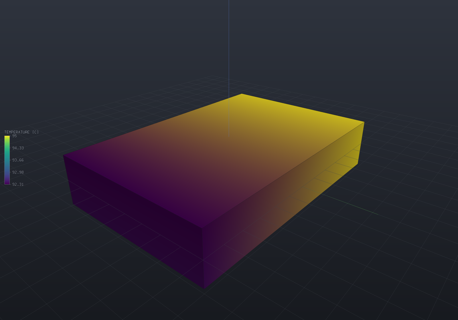

A heat spreader coloured by temperature — This example runs on the full kernel only — it uses TetMesher, which the browser build does not ship.

The left face is held at 95 °C; the top and right faces lose heat to 25 °C air through a film; every other face is unmentioned and therefore insulated. The colours are temperature, and the gradient runs left to right with the bore forcing it around — nothing is applied to the bore itself.

Units

The base system is ModelUnits’ mm / N / MPa / tonne / s, stated once on the Materials & mass page. What that implies for heat is worth a table of its own, because energy comes out as N·mm = mJ and power as mW, and two of these surprise people:

Quantity	Unit here	Against SI
Temperature	K or °C	the same (only differences matter)
Conductivity `k`	mW/(mm·K)	numerically identical to W/(m·K) — steel is 50 either way
Specific heat `c`	mm²/(s²·K)	the SI J/(kg·K) times 1e6 — steel’s 460 becomes 4.6e8
Expansion `alpha`	1/K	the same
Film coefficient `h`	mW/(mm²·K)	SI W/(m²·K) × 1e-3 — air at ~10 is 0.01 here
Heat flux	mW/mm²	SI W/m² × 1e-3
Generation	mW/mm³	SI W/m³ × 1e-6
Diffusivity `k/(rho·c)`	mm²/s	steel 13.85, i.e. SI 1.385e-5 m²/s

The conductivity coincidence is not luck — the milli- in the power cancels the milli- in the length. The specific-heat factor is the one that catches people, and Material.VolumetricHeatCapacity (steel 3.611) is the product worth sanity-checking.

Saying what is hot and what cools

Every selector from the structural page works unchanged — Facets.Tag, OnPlane, FacingAlong, InBox, All, And, Or — and the conditions map one to one:

Structural	Thermal	Meaning
`Fix` / `Prescribe`	`Temperature(selector, T)`	A held temperature (Dirichlet)
`FixNode`	`TemperatureNode(node, T)`	One node — enough to set a datum
`Pressure`	`HeatFlux(selector, q)`	Uniform flux. Positive flows INTO the body
`Force`	`HeatLoad(selector, Q)`	A total power spread over the selection — exact resultant
`Gravity`	`Generation(rate)`	Uniform volumetric generation
`BodyForce`	`Generation(p => rate)`	A generation field
`NodalForce`	`NodalHeat(node, Q)`	A point source (whose local peak does not converge)
—	`Convection(selector, h, Tinf)`	`q = h(T - Tinf)` — the one with no structural analogue

Two things have no spelling because they need none. An insulated surface is one you do not mention: zero flux is the weak form’s natural boundary condition, so an unnamed face is already adiabatic. And there is no partial restraint — a scalar field has no axes to hold separately, which is why Fix and Prescribe collapse into one call.

Convection is structurally different, not just differently named. Newton’s law of cooling has a term proportional to the unknown temperature, so it contributes to the conduction matrix as well as to the load vector. That is why it is the one condition not reduced to nodal heat when you add it: its two halves are meaningless apart. It is also what lets a model with no held temperature anywhere be solvable at all — see the refusals below.

Steady conduction

var plate = Shape.Box(80, 40, 6);
var part = new Part("plate", plate);
var surface = part.GetMesh();
var tets = TetMesher.Mesh(surface, new TetMeshOptions { RefineQuality = true, MaxElementSize = 12 });

var model = new ThermalModel(AnalysisMesh.Of(tets), Materials.Steel);
model.Temperature(Facets.OnPlane(new Vector3d(-40, 0, 0), Vector3d.UnitX), 150);
model.Convection(Facets.All, 0.02, 20);
model.Generation(0.001);                      // 1 kW per litre of resistive heating

var results = ThermalSolver.Solve(model);
Console.WriteLine(results.Report.ToText());
Console.WriteLine($"peak {results.MaxTemperature:F2} C at node {results.MaxTemperatureNode}");
Console.WriteLine($"peak heat flux {results.MaxFluxMagnitude:F1} mW/mm^2");

// The first law, discretely: heat in through sources and held boundaries must equal heat
// out through the films. It costs nothing, holds to round-off for any correct answer, and
// nothing about it is visible in a temperature plot.
if (results.Report.EnergyBalanceResidual > 1e-9)
    throw new Exception($"energy balance {results.Report.EnergyBalanceResidual:E3}");

results.WriteVtu(Path.Combine(Path.GetTempPath(), "plate-thermal.vtu"));

ThermalSolveReport is the thermal twin of FeaSolveReport: sizes, factor fill, timings, the solve residual, the temperature range, and the four heat terms — applied, through prescribed boundaries, through convection, and into storage — with the balance between them. Beyond it, ThermalResults gives nodal Temperature, averaged NodalFlux, per-material NodalFluxIn, per-element ElementFlux/ElementGradient, and TemperatureIn for a point inside an element.

Element values are public for the same reason the structural solver keeps ElementStress public: q = -k·grad T is one derivative down from the solved field, so it jumps across element faces, and the nodal values are a volume-weighted average. The size of that jump is the standard error indicator, and averaging it away is the standard way to hide a mesh that is too coarse.

At a material interface, ask for the material

Where two conductivities meet, the jump is not a discretization artefact but the answer. Temperature is continuous across a bonded interface, so the tangential gradient is continuous and the tangential flux jumps with k; only the component normal to the interface is continuous, by conservation. A node sitting on that interface therefore has one right answer per material, and NodalFlux — being indexed by node, as any colour-map field must be — holds one value and reports the blend.

// How many nodes are affected: zero for a single-material model, and for separate bodies,
// which share no node.
Console.WriteLine($"{mesh.InterfaceNodeCount} nodes blend two materials");

// The honest value, per material. Away from an interface it is bit-for-bit what NodalFlux
// says, so the two accessors are safe to mix; a region the node does not touch is refused
// by name rather than answered with a neighbour's number.
foreach (int region in mesh.RegionsAt(node))
    Console.WriteLine($"  region {region}: {results.NodalFluxIn(region, node)}");

The magnitude is worth stating: on a two-material bar carrying 5000 and 1250 mW/mm², the one value an interface node can report is wrong by 75% to 225% for one of the two materials, while NodalFluxIn is exact. StructuralResults.NodalStressIn is the same rule for the same reason.

A directional conductor

A carbon laminate conducts well along its fibres and poorly across them, so k is a tensor, not a scalar. ConductivityLaw states one — isotropic, orthotropic or fully anisotropic — with a material frame, and ThermalModel.SetConductivity sets it per region. It is the thermal twin of ElasticLaw: the same part strains orthotropically in a structural solve, so it must conduct orthotropically here, and the frame is a property of how the stuff was laid into this part rather than of the stuff, which is why the law sits beside Material rather than inside it. It is a separate type from ElasticLaw on purpose — a laminate’s conduction axes need not be its stiffness axes, so one object carrying both would make the name a claim it cannot keep.

// A laminate bar whose fibres run at 30 degrees to its long axis. The carrier states only
// density and name; the conductivity is the LAW.
var bar = Shape.Box(60, 30, 10);
var part = new Part("laminate", bar);
// Refine so the bar has INTERIOR nodes: the field below is prescribed on the whole boundary,
// so the interior is what is actually solved for.
var tets = TetMesher.Mesh(part.GetMesh(), new TetMeshOptions { RefineQuality = true, MaxElementSize = 5 });
var mesh = AnalysisMesh.Of(tets);

var carrier = new Material("carbon UD carrier", 135_000, 0.30, 1.6e-9);
double angle = 30 * Math.PI / 180;
var fibre = Frame3d.FromXY(
    Vector3d.Zero, new Vector3d(Math.Cos(angle), Math.Sin(angle), 0), Vector3d.UnitY);
var model = new ThermalModel(mesh, carrier);
model.SetConductivity(0, ConductivityLaw.Orthotropic(fibre, 40, 5, 12));   // kx, ky, kz

// A uniform temperature gradient of 2 K/mm along x on the whole boundary. The field is then
// exactly linear, so the flux is a constant vector any element reports.
const double gradient = 2.0;
foreach (int node in model.NodesOn(Facets.All))
    model.TemperatureNode(node, gradient * mesh.Position(node).X);

var results = ThermalSolver.Solve(model);
var q = results.ElementFlux(0);

Console.WriteLine($"axial conductivity  {-q.X / gradient:F2} mW/(mm.K)   (40 along fibre, 5 across)");
Console.WriteLine($"cross flux q_y      {q.Y:F2} mW/mm^2   heat carried ACROSS the gradient");
Console.WriteLine(Math.Abs(q.Y) > 1e-3
    ? "the flux is NOT parallel to the gradient -- cross-conduction, which no isotropic k can do"
    : "the flux is parallel to the gradient");

The effective axial conductivity is kx·cos²θ + ky·sin²θ — here 40·¾ + 5·¼ = 31.25, between the fibre value 40 and the transverse value 5. And the flux carries a component across the imposed gradient (the cross-conduction term), which is the one behaviour a scalar k cannot produce: an isotropic conductor’s flux is always parallel to its gradient. An anisotropic conductor’s is not, off-axis. The isotropic path is untouched — a model that states no law conducts exactly as it always did, bit for bit — and a non-symmetric or non-positive-definite tensor is refused by name, because a conductivity that let heat flow up its own gradient somewhere is unphysical.

Superconvergent flux recovery, and the error estimate

q = -k·grad T is one derivative down from the solved temperature, exactly as stress is one down from displacement, so it carries the same choice. FluxRecovery.Direct (the default) averages the element flux at each node; FluxRecovery.Superconvergent fits a polynomial per corner-node patch to the flux at the element’s superconvergent points and reads it there — the same machinery StressRecovery.Superconvergent runs, at three components rather than six, over the same (node, region) slot table. On a manufactured solution the recovered flux converges one order faster than the averaged one: measured rates 2.34 (linear) and 2.66 (quadratic) against direct evaluation’s 1.43 and 2.00, and 15× / 8× lower nodal error at the finest mesh.

The reason to build it is the estimate that comes with it. ErrorEstimate is the Zienkiewicz–Zhu figure — the energy-norm distance between the finite-element flux and its own recovery, per element and overall — which is the answer to “is this conduction mesh good enough” a solve otherwise never gives, and the per-element map an adaptive refinement loop consumes. AdaptiveSolve (see the structural page) drives that loop for the STRUCTURAL physics today; every part of it below the model — the sizing field, the gradation limiter, the budget prediction, the refusals — is physics-agnostic, so a thermal loop is the same loop with the callback returning a ThermalModel, and it is filed rather than implied.

var block = Shape.Box(60, 40, 20);
var part = new Part("block", block);
var tets = TetMesher.Mesh(part.GetMesh(), new TetMeshOptions { RefineQuality = true, MaxElementSize = 6 });

var model = new ThermalModel(AnalysisMesh.Of(tets), Materials.Steel);
model.Temperature(Facets.OnPlane(new Vector3d(-30, 0, 0), Vector3d.UnitX), 150);
model.Convection(Facets.All, 0.02, 20);
model.Generation(0.001);
var results = ThermalSolver.Solve(model);

// Is the mesh good enough? The estimate answers, and names the worst element. A large figure
// here (this is a deliberately coarse block) says: refine, and refine where WorstElement is.
Console.WriteLine(results.ErrorEstimate);       // "estimated error 43.83% (...)"
Console.WriteLine($"worst element: {results.ErrorEstimate.WorstElement}");

// The recovered flux converges one order faster; Direct stays the default so nothing moves.
results.FluxRecovery = FluxRecovery.Superconvergent;
Console.WriteLine($"peak recovered flux {results.MaxFluxMagnitude:F1} mW/mm^2");

Direct is the default for the same reason it is on the structural side: every thermal verification figure this project quotes was measured through the simple path, and a recovered field is smooth by construction — at a genuine discontinuity (a material interface, a re-entrant corner) it smooths harder than averaging does. Where no patch can be assembled at all (a mesh with no interior corner node), the estimate is NaN rather than a suspiciously-perfect zero: the honest reading is UNKNOWN, and it is the one answer that cannot be mistaken for good news.

Transient conduction

var bar = Shape.Box(40, 8, 8);
var part = new Part("quenched bar", bar);
var tets = TetMesher.Mesh(part.GetMesh(), new TetMeshOptions { RefineQuality = true, MaxElementSize = 6 });

var model = new ThermalModel(AnalysisMesh.Of(tets), Materials.Steel);
model.Temperature(Facets.OnPlane(new Vector3d(-20, 0, 0), Vector3d.UnitX), 500);

var run = ThermalSolver.SolveTransient(
    model,
    new ThermalTransientOptions(timeStep: 0.05, steps: 200)
    {
        Scheme = ThermalTimeScheme.BackwardEuler,
        InitialTemperature = 20,
        StoreEvery = 50,
    });

Console.WriteLine(run.Report.ToText());
foreach (var state in run.States)
    Console.WriteLine($"  t = {state.Time,5:F2} s: {state.MinTemperature,7:F2} to {state.MaxTemperature,7:F2} C");

Each stored state is a full ThermalResults, so flux recovery, SampleOnto and .vtu export work at any time exactly as they do for a steady solve.

The step is constant, and that is a design decision rather than a simplification: the stepping matrix C/dt + theta·K depends on the step and nothing else, so it is factored once for the whole run and every step is a back-substitution. Report.Factorizations says so. This is the “factor once, solve many right-hand sides” case that makes the direct solver’s default pay for itself — the structural solver’s own documentation notes it cannot yet claim that, and here it can.

Which scheme

	Backward Euler (default)	Crank–Nicolson
Order in time	1 (measured 1.05)	2 (measured 2.00)
Stiff modes	amplification → 0	amplification → −1: they ring
Step change	no backward move at all	swings back by up to 106% of the step

Both are unconditionally stable in the A-stable sense, but that is not the property a thermal transient needs. A conduction system’s fastest mode is roughly alpha/h², and Crank–Nicolson’s amplification factor for it approaches −1, so a sharp initial transient does not decay — it alternates sign. Measured on a 40 mm bar with 1 mm elements whose face is stepped from 20 to 100 °C (a backward step in temperature is numerical, since heat only enters):

`dt`	`lambda·dt`	Backward Euler	Crank–Nicolson
2.0 s	20	0 backward moves	190 moves, worst 105.9% (64.8% after step 5)
1.0 s	10	0 backward moves	143 moves, worst 81.5% (42.6% after step 5)
0.5 s	5	0 backward moves	242 moves, worst 56.3% (24.0% after step 5)

Use Crank–Nicolson when the transient is smooth, or when the step is short against the mesh’s own diffusion time h²/alpha — there the ringing does not arise and the second order is free.

The honest counterweight, because it is easy to over-claim here: at a short step both schemes move backwards, and that is the consistent capacity matrix, not the time integration. At dt = 0.005 s backward Euler undershoots the initial temperature by 5.8% and Crank–Nicolson by 7.1%. “Backward Euler is monotone” is true of a lumped capacity, not of this one.

Consistent capacity, and what lumping would change

The capacity matrix here is the consistent Galerkin one, integral(rho·c·N_i·N_j dV). It is what makes the measured time orders come out at theory and what lets a spatially converged transient converge at the element’s own order.

A lumped (diagonal) capacity would buy two things — a monotone answer under backward Euler, since a diagonal capacity with a positive conduction matrix gives a discrete maximum principle, and the possibility of explicit stepping, where a diagonal matrix means no solve at all. It costs accuracy: a node’s temperature becomes an average over its patch, and lumping and consistency bracket the true answer at a moving front.

What is not available is the obvious way to lump. Row-sum lumping sets C_ii = sum_j C_ij = rho·c·integral(N_i dV), which for a 10-node tetrahedron is −V/20 at every corner node — a negative heat capacity, a node that cools when heated. It is the same integral, and the same surprising number, that a quadratic element’s gravity load already has. Any lumping for quadratic elements has to be a scaled-diagonal scheme instead, which is a different approximation with its own error, so it is filed rather than smuggled in under one name.

Thermal stress

A temperature field becomes a thermal-expansion load on a structural model over the same mesh:

var bar = Shape.Box(60, 20, 10);
var part = new Part("restrained bar", bar);
var tets = TetMesher.Mesh(part.GetMesh(), new TetMeshOptions { RefineQuality = true, MaxElementSize = 10 });
var mesh = AnalysisMesh.Of(tets);
var steel = Materials.Steel;

// One conduction solve...
var thermal = new ThermalModel(mesh, steel);
thermal.Temperature(Facets.OnPlane(new Vector3d(-30, 0, 0), Vector3d.UnitX), 120);
thermal.Temperature(Facets.OnPlane(new Vector3d(30, 0, 0), Vector3d.UnitX), 120);
var temperature = ThermalSolver.Solve(thermal);

// ...driving one structural solve. Held against axial growth at both ends, and on rollers
// at one y face and one z face so the bar is still free to grow sideways.
var structural = new StructuralModel(mesh, steel);
structural.Fix(Facets.OnPlane(new Vector3d(-30, 0, 0), Vector3d.UnitX), Dof.X);
structural.Fix(Facets.OnPlane(new Vector3d(30, 0, 0), Vector3d.UnitX), Dof.X);
structural.Fix(Facets.OnPlane(new Vector3d(0, -10, 0), Vector3d.UnitY), Dof.Y);
structural.Fix(Facets.OnPlane(new Vector3d(0, 0, -5), Vector3d.UnitZ), Dof.Z);
structural.ThermalLoad(temperature, referenceTemperature: 20);

var results = StructuralSolver.Solve(structural);

double expected = -steel.YoungsModulus * steel.ThermalExpansion * (120 - 20);
Console.WriteLine($"sigma_xx measured {results.ElementStress(0).Xx:F3} MPa");
Console.WriteLine($"        -E.alpha.dT {expected:F3} MPa");

Two halves make that work, and forgetting the second is the classic way to get thermal stress wrong. The load is integral(B' · D · eps0), which for an isotropic material collapses to E/(1-2·nu)·alpha·dT times a shape-function gradient. The stress recovery must then use sigma = D(eps - eps0), not D·eps — a bar free to expand develops the full thermal strain and carries zero stress, and without the subtraction it would report E·alpha·dT (126 MPa for steel at a 50 K rise) on a body under no load at all. Both halves come from one stored field, so applying the load is what turns the subtraction on and there is no second call to forget.

A thermal load is self-equilibrated by construction — the shape functions are a partition of unity, so their gradients sum to exactly zero — which means it adds nothing to the applied resultant and the solver’s equilibrium check keeps its meaning through a coupled solve.

[!NOTE] The two models must share the same AnalysisMesh instance, and that is checked. A temperature field crosses by node index, and two meshes of the same body can number their nodes differently, so the alternative is applying each node’s temperature to some other node — a plausible wrong answer, which is the one outcome worth refusing.

Refusals

An undriven body is refused before the factorization, per connected body:

The model has no prescribed temperature and no convective surface, so its conduction
matrix is singular: adding any constant to the temperature everywhere leaves every
gradient, and therefore every heat flux and every boundary condition, exactly as it was.
There is no unique answer to return, and a field that merely looked reasonable would be
wrong by an unknowable offset. Prescribe a temperature somewhere (one node is enough to
set the datum), or give a surface a convective condition.

This is conduction’s analogue of an unrestrained structural body, and it is both simpler and sharper. The conduction operator’s null space on a connected body is exactly the constants, so the check is a boolean — is there a held temperature or a convective facet anywhere? — where the structural check needs an eigen-decomposition to find which of six rigid modes partly survive. A pure heat flux does not count: it is a Neumann condition and says nothing about the level. If heat is going in with nowhere to leave, the message says that too, because no steady state exists at all and a transient is the honest model.

A transient of a perfectly insulated body is not refused: the capacity term is positive definite on its own, so it removes the constant null space the steady operator has. The body holds its energy, which is the right answer.

Also refused by name: a material with no conductivity (the matrix would be identically zero — the answer would not be inaccurate, it would not exist); a transient on a material with no heat capacity, pointing at the steady solver, since a body with no capacity is its steady state; a selector matching no facets, naming the tags that do exist; a non-positive film coefficient, explaining that zero is not a condition and a negative one would make the matrix indefinite; every node prescribed; and a thermal load whose field is the wrong length, naming the quadratic mid-edge nodes that are usually the cause.

Verification

A solver is worth exactly what its verification is worth, so here is all of it. Every number is from tests/EngrCAD.Fea.Tests, on structured meshes so a measured convergence order means something.

Element matrices against closed forms and independent quadrature rules:

Check	Measured
Conductivity annihilates a constant field (both orders)	1.1e-16 / 1.6e-16
4-node conductivity vs `k·V·grad L_i · grad L_j`	7.1e-15
4-node capacity vs `rho·c·V/20 · (2, 1)`	2.2e-16
Capacity row sums vs `rho·c·integral(N_i dV)`	6.7e-16 / 1.1e-14
3-node convection matrix vs `h·A/12 · (2, 1)`	1.0e-17
6-node convection, degree 4 vs degree 5	9.9e-16
Thermal-expansion load sums to zero (both orders)	5.6e-15 / 1.7e-14

Each “the cheap rule is exact” claim has a negative control, because two rules agreeing proves nothing if the code ignores the rule it was handed:

Quadratic conductivity, degree 2 vs degree 3: 1.1e-15 straight-sided, and 3.0e-2 when one mid-edge node is moved off the midpoint. The exactness really is the straight-sidedness.
Linear capacity with the conductivity’s one-point rule: every entry is rho·c·V/16 (spread exactly 0), so the matrix is rank one and singular — while its total is rho·c·V to 1e-14. A “does the capacity sum right” check passes it.
Under-integrating the generation load with a degree-1 rule instead of degree 5: 1.28e3× worse (7.8e-1 against 6.1e-4).

Steady solutions — three of the five are exact to round-off, which is why they were chosen: a linear field, and the linear field a slab with a convective end settles into, lie inside both element spaces.

Case	Linear	Quadratic
Patch test (linear field, temperature)	2.4e-16	7.3e-16
Patch test (element flux)	2.3e-15	8.0e-15
1D slab, fixed faces, vs the linear profile	1.4e-15	3.8e-15
1D slab, heat through vs `k·A·dT/L`	4.7e-16	1.5e-15
Slab with generation, nodal, vs the parabola	8.8e-14	1.4e-13
Convective face, vs the mixed-BC solution	9.0e-14	3.9e-13
Convective face, heat out vs `h·A(Ts − Tinf)`	2.6e-15	1.1e-14

The generation case carries a lesson. Both orders are nodally exact, for two different reasons — a parabola is in the quadratic space, and linear elements have the classical one-dimensional nodal superconvergence (the discrete equations reduce to a central difference, which a quadratic satisfies with no truncation error). Measuring “the error” at nodes therefore reports round-off at every refinement and no order at all; the first version of that test asserted a ratio of 4 and measured 0.72, which is the ratio of two numbers that are both nothing. The genuine O(h²) is inside the elements, and measured there the ratio is 4.00, 4.00.

Radial, a hollow cylinder against T(r) = Ta + (Tb − Ta)·ln(r/a)/ln(b/a):

	nRadial 2	4	8	order
Linear	5.3e-3	2.4e-3	1.0e-3	1.28
Quadratic	9.4e-3	2.3e-3	5.8e-4	2.00

Both are below theory (2 and 3), and the cause is measured rather than guessed: the fixture’s rings are polygons, so refining the mesh refines the domain too, and the boundary condition is constant along each chord where the true logarithmic profile is not. Refining the angular direction as n² instead of n — which drops the chord sagitta from O(h²) to O(h⁴) — lifts quadratic to 2.28 and its finest error to 1.1e-4, while leaving the linear sequence unchanged at 1.28 and 1.0e-3. So the two are limited by different things: the quadratic element is good enough that the polygonal boundary holds it back, and the linear one is still limited by its own radial approximation.

There is a fixture trap here worth keeping. Spacing the rings geometrically makes the nodal values exact (4.3e-14 on a 120 K drop at every refinement), because the nodes then sit at equal intervals of ln r and every ring-to-ring conductance is equal — so the exact values satisfy the discrete equations identically. The first version of that study reported convergence orders of −2.50 and −1.27, which is what a ratio of two round-off figures looks like when mistaken for a signal.

Convergence order by the method of manufactured solutions, on a box the mesh represents exactly:

	L2 measured	theory	energy measured	theory
Linear	2.01	2	1.00	1
Quadratic	3.05	3	2.02	2

The manufactured field is quartic, and that is a trap the suite walked into with a cubic one first: a cubic field on a uniform mesh is reproduced exactly at the nodes by both element types, because the stencil’s truncation error is proportional to a fourth derivative a cubic does not have. The study then reports round-off (2.2e-13 on a field of scale 113) and no order whatsoever.

Transient:

Check	Measured
Lumped capacitance vs `Tinf + (T0−Tinf)·exp(−t/tau)`, Bi = 2.1e-3	3.0e-4 / 5.3e-4 of the initial excess
Semi-infinite solid vs the erfc profile (h = 1 mm, dt = 5 ms)	0.184 K on an 80 K step, 2.3e-3
Transient run to 20 tau vs the steady solve	3.4e-9 relative
Time order, backward Euler	1.05 (theory 1)
Time order, Crank–Nicolson	2.00 (theory 2)
First law over a whole run	1.3e-14 … 8.5e-13
Insulated body’s stored energy over 10 steps	drift < 1e-14

The time order is measured against a reference solve of the same semi-discrete system, not against the analytic exponential: comparing to the latter folds the spatial discretization into the error and caps the measured order at whatever the mesh contributes. The step range also has to put every mode in the asymptotic regime — run over a full time constant with eight steps, Crank–Nicolson reported 1.80, 3.72 and 3.21 across one sequence, a genuine sign change in the error rather than noise.

Coupling — both bars are exact to round-off, which is why they were chosen: the free bar’s answer is a linear displacement field and the constrained bar’s a uniform strain state, so both lie inside both element spaces and there is no discretization error to hide a factor-of-two in.

Check	Linear	Quadratic
Free bar, expansion `alpha·dT·L`	6.9e-15	8.7e-15
Free bar, stress (must vanish) vs `E·alpha·dT`	8.5e-15	3.6e-14
Constrained bar, `sigma_xx` vs `−E·alpha·dT`	2.0e-15	5.0e-15
Constrained bar, `sigma_yy`/`sigma_zz` (must vanish)	5.8e-13 MPa	1.0e-12 MPa
Constrained bar, lateral growth vs `beta·y`	3.1e-18	1.0e-17
Stress linear and correctly signed at dT = −40, −5, 5, 80	1.3e-15	—

The constrained bar is the case that catches a wrong modulus: it is independent of length and of Poisson’s ratio, so a coupling using E where it should use E/(1−2·nu) gets the free bar right and this one wrong by 2.5 at nu = 0.3.

A coupled pipeline check adds one more, and it carries its own trap. A linear temperature field is stress-free in an unconstrained body — that is the exact condition, since Saint-Venant compatibility forces every second derivative of dT to vanish — but the stress-free displacement field is quadratic: u_x needs a −(b/2)(y² + z²) term to cancel a shear the obvious guess introduces. Which means whole symmetry planes over-constrain it, and the model then genuinely carries stress from the restraints alone (measured 67 MPa, a quarter of E·alpha·dT). A statically determinate 3-2-1 restraint gives 1e-10.

Limitations

Temperature-dependent properties are a separate solver (ThermalNonlinear.Solve for steady k(T), ThermalNonlinear.SolveTransient for c(T) and per-step k(T), below); the LINEAR solve keeps constant properties by design — that is what makes it one factorization. The expansion alpha stays constant everywhere.
A transient streams when asked: OnState sees exactly the states a retained run stores (bit-identical, asserted against a retained twin) and RetainStates = false caps the returned list at the two ends — a run of any length writes each state to a .vtu and discards it.
The time STEP is constant, deliberately: it is what makes one factorization serve the whole run. Time-varying boundary values are first-class (the law overloads above); a time-varying step is the different, much larger change.
The capacity matrix is consistent by default, with lumping a named option (ThermalTransientOptions.Lumping = MassLumping.Hrz): at steps short against the element diffusion time the consistent capacity violates the discrete maximum principle — measured on the quench fixture, the node next to the quenched face is pushed above the initial temperature — and the lumped diagonal restores it (backward Euler becomes an M-matrix step; nothing leaves [surface, initial]). HRZ preserves each element’s capacity exactly and coincides with row-sum on 4-node elements to round-off; row-sum on 10-node elements is refused by name (−V/20 at every corner — a negative heat capacity).
Sliver elements are the real constraint, and they belong to the mesher — the same limitation the structural page records, refused by name here by the same shared guard.

Temperature-dependent conductivity

ThermalNonlinear.Solve(model, conductivityByRegion) handles k = k(T) as the second consumer of the outer-iteration shape radiation established — with the one structural difference stated up front: a radiating pass moves only the load, while a conductivity pass changes the matrix, so every iteration re-assembles and re-factors. Each pass evaluates the law per element at the element’s node-mean temperature from the previous answer; a converged fixed point solves the true k(T) problem in the per-element-constant sense the discretization carries anyway. Regions not named keep their constant conductivity (a directional ConductivityLaw cannot also take a temperature law — that composition is a temperature-dependent tensor, a different feature, refused by name).

The oracle is the Kirchhoff transform: for k(T) = k0(1 + βT) the variable θ = ∫k dT is linear in x, so a slab held at T1/T2 carries flux q = (k0/L)[(T1 − T2) + β(T1² − T2²)/2] exactly — a closed form sharing no line with the solver’s linearization. One caveat is stated rather than discovered: the returned results’ flux accessors read the model’s constant laws (the overlay is cleared when the solve returns), so the converged per-element k rides on the result (ElementConductivity) and the nonlinear flux is the accessor’s value rescaled by it.

var bar = Shape.Box(40, 8, 8).Translate(20, 0, 0);
// Refined: with BOTH ends held, a minimal box mesh would leave no free node at all.
var mesh = AnalysisMesh.Of(TetMesher.Mesh(bar.ToMesh(),
    new TetMeshOptions { MaxElementSize = 5, RefineQuality = true }));
var model = new ThermalModel(mesh, Materials.Aluminium6061)
    .Temperature(Facets.OnPlane(Vector3d.Zero, new Vector3d(-1, 0, 0)), 0.0)
    .Temperature(Facets.OnPlane(new Vector3d(40, 0, 0), Vector3d.UnitX), 100.0);
const double k0 = 167, beta = 0.01;
var run = ThermalNonlinear.Solve(model,
    new Dictionary<int, Func<double, double>> { [0] = t => k0 * (1 + beta * t) });

// Kirchhoff: q = (k0/L)[(T1 − T2) + beta(T1² − T2²)/2].
double exact = k0 / 40 * (100 + beta * 100 * 100 / 2);
double flux = 0;
for (int e = 0; e < mesh.ElementCount; e++)
    flux += Math.Abs(run.Results.ElementFlux(e).X) * run.ElementConductivity[e] / k0;
flux /= mesh.ElementCount;
Console.WriteLine($"flux {flux:0.0} vs Kirchhoff {exact:0.0} mW/mm2 "
    + $"in {run.Iterations} iterations");

The property-nonlinear transient: c(T) and k(T) per step

ThermalNonlinear.SolveTransient(model, transient, conductivityByRegion?, capacityByRegion?) steps a transient whose properties follow the temperature — a sequence of one-step constant-property transients, each evaluating the laws per element at the step’s start temperatures and running the linear stepper seeded from the previous state. The composition reuses the stepping machinery verbatim (schemes, lumping, prescribed snapping, the per-step first-law identity), and it states the cost honestly: a property nonlinearity re-assembles and re-factors every step (Factorizations equals the step count by construction) — exactly the one-factorization amortisation the linear transient celebrates and this one necessarily gives up. The capacity law returns the specific heat c(T) (the datasheet quantity); laws returning the material’s own constants reproduce the plain transient bit for bit — and time-varying load and prescribed laws compose too: a sub-run’s clock restarts at zero, so its laws are re-based to the run’s own instants internally, and a constant-property run carrying a ramped flux and a ramped prescribed temperature reproduces the plain lawed transient bit for bit at a dyadic step (the re-based instant (n−1)·dt + dt and the plain run’s n·dt agree exactly only where dt’s products are exact; a general step differs by its own ulp — a wrong offset would shift the ramp by whole steps).

The oracle is an identity, not a convergence claim: an insulated cube under uniform generation stays spatially uniform (the generation load and the capacity rows share the partition-of-unity weights), so the FE step reduces exactly to the scalar recurrence T ← T + dt·g/(ρc(T)) — and as the step shrinks, that recurrence converges on the enthalpy closed form ρ(c0·T + c0γT²/2) = g·t at first order, matching backward Euler’s own.

var cube = Shape.Box(8, 8, 8).Translate(4, 4, 4);
var mesh = AnalysisMesh.Of(TetMesher.Mesh(cube.ToMesh()));
var model = new ThermalModel(mesh, Materials.Aluminium6061).Generation(2.0);
double c0 = Materials.Aluminium6061.SpecificHeat;
var run = ThermalNonlinear.SolveTransient(
    model, new ThermalTransientOptions(0.5, 20),
    capacityByRegion: new Dictionary<int, Func<double, double>>
    {
        [0] = t => c0 * (1 + 0.002 * t),   // c grows 0.2 %/K
    });
Console.WriteLine($"T(10 s) = {run.States[^1].Temperature[0]:0.000} K over "
    + $"{run.Factorizations} factorizations (one per step, the honest cost)");

Surface radiation

ThermalRadiation.Solve(model, surfaces) adds grey-body radiation, q = σ·ε·(T⁴ − Ts⁴), as the outer iteration the conduction model’s own remarks reserve for it — the fourth power is nonlinear in the unknown and everything else here is one factorization. Each pass linearizes per facet about the previous answer’s facet mean, h_rad = σ·ε·(T̄² + Ts²)(T̄ + Ts) with ambient Ts — exactly a convective film, assembled by the same surface quadrature — and the linearization is exact at its own point, so a converged answer satisfies the true Stefan–Boltzmann balance. The plain Picard map was measured oscillating in a limit cycle, so the linearization point is under-relaxed (half steps by default); a radiating facet counts as driven, so a model held by nothing but its own glow is solvable.

Temperatures must be absolute (kelvin): a model built in celsius is silently wrong physics no solver can detect, which is why a non-positive surrounding refuses loudly.

// A generating cube radiating to 300 K surroundings: the equilibrium is the lumped
// Stefan-Boltzmann closed form, solved here independently by bisection on the balance.
var cube = Shape.Box(10, 10, 10);
var mesh = AnalysisMesh.Of(TetMesher.Mesh(cube.ToMesh()));
const double emissivity = 0.8, surroundings = 300, power = 1500; // mW
var model = new ThermalModel(mesh, Materials.Aluminium6061)
    .Generation(power / 1000.0);
var run = ThermalRadiation.Solve(model,
    [new RadiationSurface(Facets.All, emissivity, surroundings)]);

double sigmaEps = ThermalRadiation.StefanBoltzmann * emissivity;
double lo = surroundings, hi = 3000;
for (int i = 0; i < 200; i++)
{
    double mid = 0.5 * (lo + hi);
    if (sigmaEps * 600 * (Math.Pow(mid, 4) - Math.Pow(surroundings, 4)) < power) lo = mid;
    else hi = mid;
}
Console.WriteLine($"radiating equilibrium {run.Results.Temperature.Average():0.00} K "
    + $"vs the closed form {0.5 * (lo + hi):0.00} K in {run.Iterations} iterations");

Time-varying boundary conditions

Every load condition takes a time law overload — HeatFlux(facets, t => ...), HeatLoad(facets, t => ...), Convection(facets, h, t => ambient), Temperature(facets, t => ...) — for the ramped platen, the duty-cycled component, the day–night ambient. A law moves only the load: the spatial pattern is assembled once at add time (at unit law value) and scaled at each instant the transient samples, so the single-factorization contract survives untouched. The film coefficient stays constant and that is a stated boundary, not an omission — h enters the matrix, which is factored once, while the ambient enters only the supply. A steady solve refuses a law-carrying model by name (it has no time to hand it), and the energy balance keeps the split the constant conditions live by: an applied law joins the applied heat, an ambient law joins the convective supply.

The oracle with teeth is discrete exactness: for a prescribed ramp R·t the discrete particular solution is a·t + b with a the uniform vector R and K·b = −M·a — which makes b the steady solver’s own answer for a uniform generation of −ρc·R held at zero — and any theta scheme integrates a linear-in-time particular solution exactly. Seed the run with b and every step must land on b + R·t to round-off, backward Euler and Crank–Nicolson alike:

var bar = Shape.Box(20, 8, 8).Translate(10, 0, 0);
var tets = TetMesher.Mesh(bar.ToMesh());
var mesh = AnalysisMesh.Of(tets);
var metal = Materials.Aluminium6061;
double rhoC = metal.Density * metal.SpecificHeat;
const double rampRate = 3.0;

// b: the steady answer for generation −ρc·R with the ramped face held at law(0) = 0.
var b = ThermalSolver.Solve(new ThermalModel(mesh, metal)
    .Temperature(Facets.OnPlane(Vector3d.Zero, new Vector3d(-1, 0, 0)), 0.0)
    .Generation(-rhoC * rampRate));

var model = new ThermalModel(mesh, metal)
    .Temperature(Facets.OnPlane(Vector3d.Zero, new Vector3d(-1, 0, 0)), t => rampRate * t);
var run = ThermalSolver.SolveTransient(model,
    new ThermalTransientOptions(0.5, 8) { InitialField = [.. b.Temperature] });

double worst = 0;
foreach (var state in run.States)
    for (int node = 0; node < mesh.NodeCount; node++)
        worst = Math.Max(worst,
            Math.Abs(state.Temperature[node] - (b.Temperature[node] + rampRate * state.Time)));
Console.WriteLine($"worst |T − (b + R·t)| over the whole run: {worst:E2}");
if (worst > 1e-8)
    throw new Exception("the linear particular solution must integrate exactly");

Heatsink sizing (correlations checked by the solver)

HeatsinkSizing.Size is the spreadsheet a natural-convection heatsink is chosen by, with the one thing no spreadsheet has: the answer can be checked against this repo’s own thermal FEA. The sizing side is closed form — the Bar-Cohen & Rohsenow composite Nusselt correlation with the Elenbaas optimum spacing (El = 54.3; the classic Nu = 1.31 is derived from the composite rather than stored), fin efficiency tanh(mH)/(mH), dry-air properties at 300 K — every constant a ⚠ verify-against-datasheet transcription asserted in datasheet form. Fin-array sizing is vertical fins only (the transcribed case, offered by name); forced convection wants a stated film coefficient.

Horizontal flat plates are transcribed too — the McAdams family over the A/P characteristic length: heated-facing-up Nu = 0.54·Ra^(1/4) (laminar) and 0.15·Ra^(1/3) (turbulent), heated-facing-down 0.27·Ra^(1/4), each valid only in its own Rayleigh range and refused by name outside it (a correlation is a fit; outside its data it is a guess wearing four significant figures). Two identities carry the verification: facing-up is exactly twice facing-down in the shared laminar range (0.54 = 2 × 0.27, and doubling commutes with rounding, so the ratio is bit-exact), and the turbulent ⅓ power cancels the L³ inside Ra, so the film coefficient is independent of the plate’s size — two different plates read one h, the identity a wrong exponent cannot fake.

var up = NaturalConvection.PlateFacing.HeatedFacingUp;
var down = NaturalConvection.PlateFacing.HeatedFacingDown;
// A 150 mm square plate 50 K above ambient (SI at the correlation boundary; large
// enough that its Rayleigh number ~2e5 sits inside BOTH quarter-power ranges — a
// 100 mm plate's 7e4 is refused by the facing-down correlation's own 1e5 floor).
double h = NaturalConvection.PlateFilmCoefficient(50, 0.0225, 0.6, up);
Console.WriteLine($"150 mm plate, heated face up:  h = {h:0.00} W/(m2 K)");
Console.WriteLine($"same plate, heated face down:  h = "
    + $"{NaturalConvection.PlateFilmCoefficient(50, 0.0225, 0.6, down):0.00} (half)");
Console.WriteLine($"1 m and 2 m plates, turbulent: "
    + $"{NaturalConvection.PlateFilmCoefficient(50, 1, 4, up):0.000} vs "
    + $"{NaturalConvection.PlateFilmCoefficient(50, 4, 8, up):0.000} (size cancels)");

var spec = new HeatsinkSpec(
    PowerWatts: 12, AllowableRise: 35, BaseWidth: 80, BaseDepth: 80, MaxFinHeight: 40);
var design = HeatsinkSizing.Size(spec);
Console.WriteLine($"{design.FinCount} fins at {design.FinSpacing:0.0} mm spacing, "
    + $"height {design.FinHeight:0.0} mm");
Console.WriteLine($"h = {design.FilmCoefficient:0.0} W/(m2 K), eta = {design.FinEfficiency:0.000}, "
    + $"R = {design.ThermalResistance:0.00} K/W -> rise {design.PredictedRise:0.0} K");

// The solid the design describes: a base plate plus the fin pattern - the geometry is
// the easy half in this kernel.
var sink = Shape.Box(spec.BaseWidth, spec.BaseDepth, spec.BaseThickness);
double pitch = design.FinSpacing + spec.FinThickness;
double firstX = -(design.FinCount - 1) * pitch / 2;
var fin = Shape.Box(spec.FinThickness, spec.BaseDepth, design.FinHeight)
    .Translate(firstX, 0, (spec.BaseThickness + design.FinHeight) / 2);
sink = sink | fin.PatternLinear(design.FinCount, new Vector3d(pitch, 0, 0));
Console.WriteLine($"solid: {sink.ToMesh().FaceCount} facets, "
    + $"volume {sink.ToMesh().Volume():0} mm^3");

Closing the loop: a parametric heatsink under a design study

The follow-up the sizing tool invites: put the heatsink in a feature history and let a design study drive it. The layering is deliberate — EngrCAD.Modeling cannot reference EngrCAD.Fea, so a Feature cannot call HeatsinkSizing; the composition lives at the application layer, where the objective and constraint read the correlations directly. And the loop is instant, because of a recorded design fact: a Shape graph is lazy, so regenerating a part costs nothing until something measures it — the study below runs ~380 evaluations in milliseconds, reading closed forms, and the geometry is measured once, at the winner, where the generated solid’s mass must agree with the closed form the study reasoned with.

// Minimise mass subject to a thermal-resistance limit (12 W at a 35 K rise). The study
// STARTS infeasible (the default design reads ~4 K/W) and climbs in, ending exactly ON
// the constraint.
sealed class FinnedSink : Feature
{
    public const double Width = 80, Depth = 80, FinThickness = 2, BaseThickness = 4;

    [Param(Min = 8, Max = 40, Units = "mm")] public double FinHeight { get; init; } = 25;
    [Param(Min = 4, Max = 14, Units = "mm")] public double FinSpacing { get; init; } = 6;

    public int FinCount =>
        (int)Math.Floor((Width - FinThickness) / (FinSpacing + FinThickness)) + 1;

    public override Shape Apply(FeatureContext c)
    {
        double pitch = FinSpacing + FinThickness;
        var plate = Shape.Box(Width, Depth, BaseThickness);
        var fin = Shape.Box(FinThickness, Depth, FinHeight)
            .Translate(-(FinCount - 1) * pitch / 2, 0, (BaseThickness + FinHeight) / 2);
        return plate | fin.PatternLinear(FinCount, new Vector3d(pitch, 0, 0));
    }
}

var sink = new FinnedSink();
var history = new FeatureHistory();
history.Add(sink);
var part = history.ToPart("sink").Of(Materials.Aluminium6061);

double ClosedFormMassGrams(FinnedSink f) =>
    (FinnedSink.Width * FinnedSink.Depth * FinnedSink.BaseThickness
        + f.FinCount * FinnedSink.FinThickness * FinnedSink.Depth * f.FinHeight)
    * 2.70e-9 * 1e6;

double Resistance(FinnedSink f)
{
    const double rise = 35, ambient = 300;
    double s = f.FinSpacing / 1000, length = FinnedSink.Depth / 1000;
    double el = 9.81 * (1 / (ambient + rise / 2)) * rise * s * s * s * s
        / (NaturalConvection.AirKinematicViscosity
            * NaturalConvection.AirThermalDiffusivity * length);
    double h = NaturalConvection.Nusselt(el) * NaturalConvection.AirConductivity / s;
    double eta = NaturalConvection.FinEfficiency(
        h, 167, FinnedSink.FinThickness / 1000, f.FinHeight / 1000);
    double area = f.FinCount * 2 * (f.FinHeight / 1000) * length * eta
        + (FinnedSink.Width / 1000) * length;
    return 1 / (h * area);
}

double Mass(Part p) => ClosedFormMassGrams((FinnedSink)p.History!.Features[0]);
double R(Part p) => Resistance((FinnedSink)p.History!.Features[0]);

var height = DesignVariable.On(sink, nameof(FinnedSink.FinHeight));
var spacing = DesignVariable.On(sink, nameof(FinnedSink.FinSpacing));
var result = DesignStudy.Minimize(
    part, [height, spacing], Mass,
    [StudyConstraint.AtMost("thermal resistance", R, 35.0 / 12)]);
Console.WriteLine(result.Report());

// The loop closure: the solid the winner describes, MEASURED, against the closed form
// the study reasoned with — one mesh, at the answer only.
var winner = new FinnedSink
{
    FinHeight = result.ValueOf(height),
    FinSpacing = result.ValueOf(spacing),
};
var winnerHistory = new FeatureHistory();
winnerHistory.Add(winner);
double measured = winnerHistory.ToPart("winner").Of(Materials.Aluminium6061).MassGrams()!.Value;
double closed = ClosedFormMassGrams(winner);
Console.WriteLine($"winner {winner.FinCount} fins x {winner.FinHeight:0.0} mm: "
    + $"measured {measured:0.0} g vs closed form {closed:0.0} g");

if (Resistance(new FinnedSink()) <= 35.0 / 12)
    throw new Exception("the default design should START infeasible");
if (!result.Feasible)
    throw new Exception("no feasible design found");
if (result.Stop.BindingConstraints is not ["thermal resistance"])
    throw new Exception("the resistance limit should be what stopped the search");
if (Math.Abs(measured - closed) / closed > 0.01)
    throw new Exception($"the generated solid disagrees with the study's closed form");

The verification is the deliverable: the fin-efficiency closed form is held against an independent finite-difference solve of the 1D fin equation (equal to eight digits), and — the discriminating row — against a real 3D conduction solve of the same fin through ThermalSolver’s own Convection film BCs: base held at the rise, the film on the two faces, tip adiabatic so both constructions describe one fin. Measured: η = 0.959, closed form 2.2105 W against FEA 2.2107 W — ratio 1.0001. The Elenbaas spacing carries its own quarter-power scalings (S(16L) = 2·S(L) to twelve digits), and an envelope that cannot meet the rise refuses naming both the asked and the achievable power.